On our site you often read about this „geospatial data” thing. I thought that since we mentioned it so frequently, I dedicated a whole article to it. In it I sum up what you need to know about these data, how you can classify them and how they’re being used. I also add a „how to” section with exact software tutorials. All presented software are free to use so you can try all the described methods and techniques. I recommend this article for those who are only getting into mapping and modeling.

I think this will be very useful for beginner drone users because from this article you can learn how to create cartographically correct road network, estate records, land cover maps by using orthophotos. Or how to create slope and aspect maps.

Be prepared because this is going to be a long but hopefully instructive read. 🙂

What is geospatial data?

In a nutshell, geospatial data are any data that have connection to an exact place in geometrical terms. Okay…I said that it’s gonna be a long read so I’m not taking it brief. A geospatial data can be a coordinate or a location which we can position in space. Also, aerial photos, digital elevation models (DEM), satellite images, LIDAR point clouds, plot boundary maps belong to the category of geospatial data. Of course, I won’t mention all of them but now you have a clue about what we are dealing with here. Geospatial data can be divided into two groups based on data models: vector and raster. In case of vector files, we display the geometrical elements (points, lines, polygons, solids) by coordinates ordered to vertices. Meanwhile when we use a raster data model, we cover the surface like a mosaic. These covering elements can be triangles, squares, hexagons.

“Which model should I use?” you might ask. Well, it depends on the nature of data collection and on the goal of the work. Creating a vector file can be a bit complicated because you must plan the geometry itself. Also, you need to create the attribute table and even fill it with data if needed. Storing vector data is also less problematic since it doesn’t require that much storage compared to the raster model.

Sidenote: The statement about the storage requirements is only partly true because a point cloud is also a vector data model and these files can be huge.

Raster files can be created on an easier and quicker way however with these files you can only achieve an exact display because every cell can contain only one type of data. If you would like to read more about vectors I recommend this article.

If you are interested in raster and you want to really dig into the basics of geospatial data then I recommend this article.

Vectorgraphical data

The fact, my dear Reader, is that If I wanted to present all data types in the needed depth, then you wouldn’t have time to read our other magnificent articles.

Now we will be talking about creating a shapefile which is the most common GIS format. Also, I will show you how you can create map-content by using this shapefile and how you can shape this in 3D. At the end I will also show you how to convert a 3D file into a point cloud and I will also make a special measurement. 

Creating shapefile

Before we get started it is important to mention that the software I use in this section is called QGIS 3.22.1. It’s a free software so feel free to download it and try it out.

If you open QGIS after installing you will see the following.

Choose “New Empty Project”. Be very careful with coordinate systems and transformations when using this software. Here you find them in EPSG (European Petroleum Survey Group) code formats, for example 4326=WGS84. GPS, GNSS and UAV also use this.Add a base map to our map, so we will always know where we are located in space. Of course, this basic map can be an orthophoto map made by drone. If you look up the orthophoto in the sidebar on the left hand side you just easily drag-and-drop it to the map. If you don’t have your own base map you choose “XYZ Tiles” on the left sidebar then double-click to the “OpenStreetMap” option.

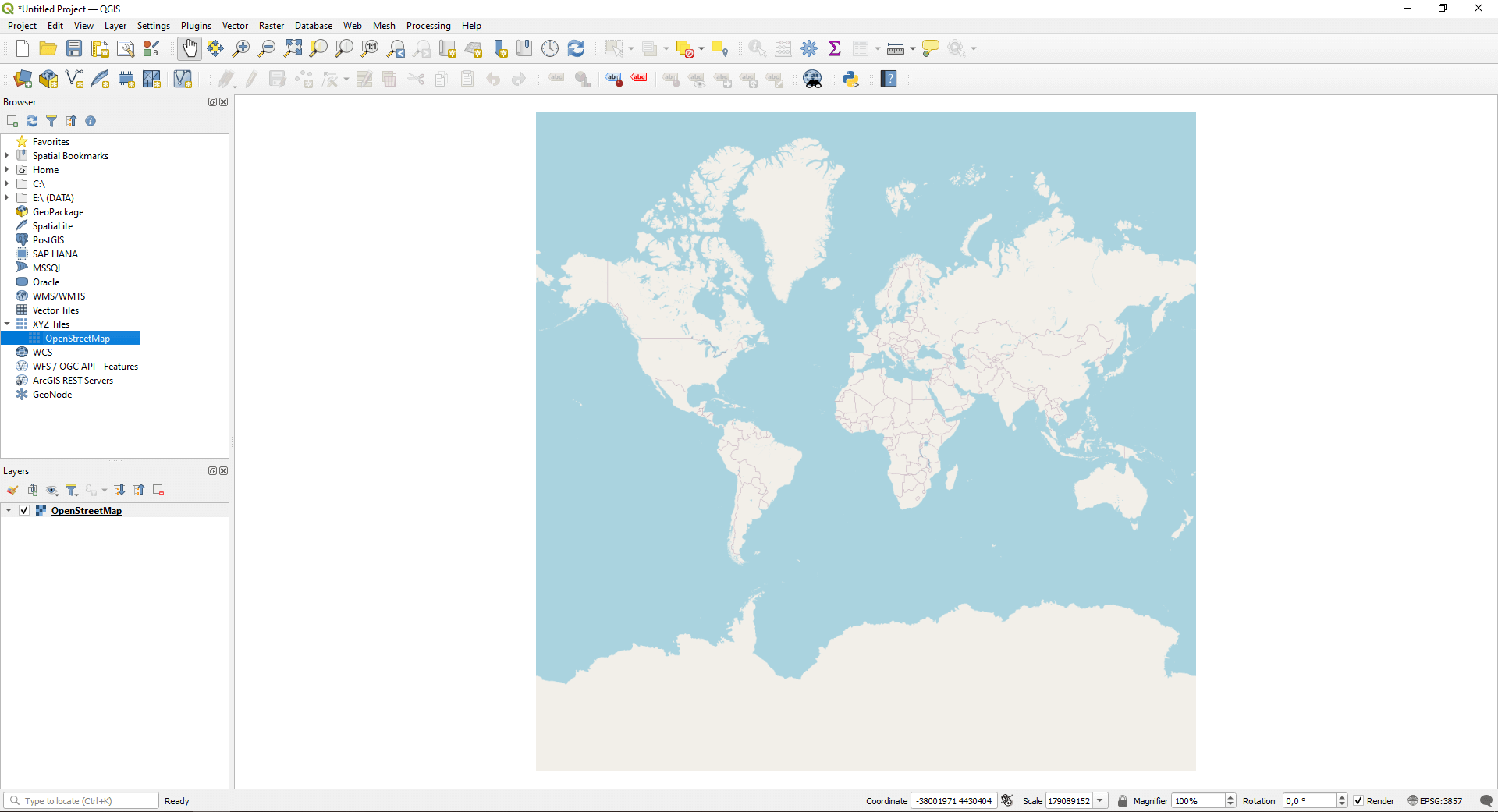
If you are attentive, you can notice that in the bottom right corner the EPSG code changed from 4326 to 3857. This change happened because most of the web-based maps (e.g. OneStreetMap) are using the “Pseudo-Mercator  coordinate system.

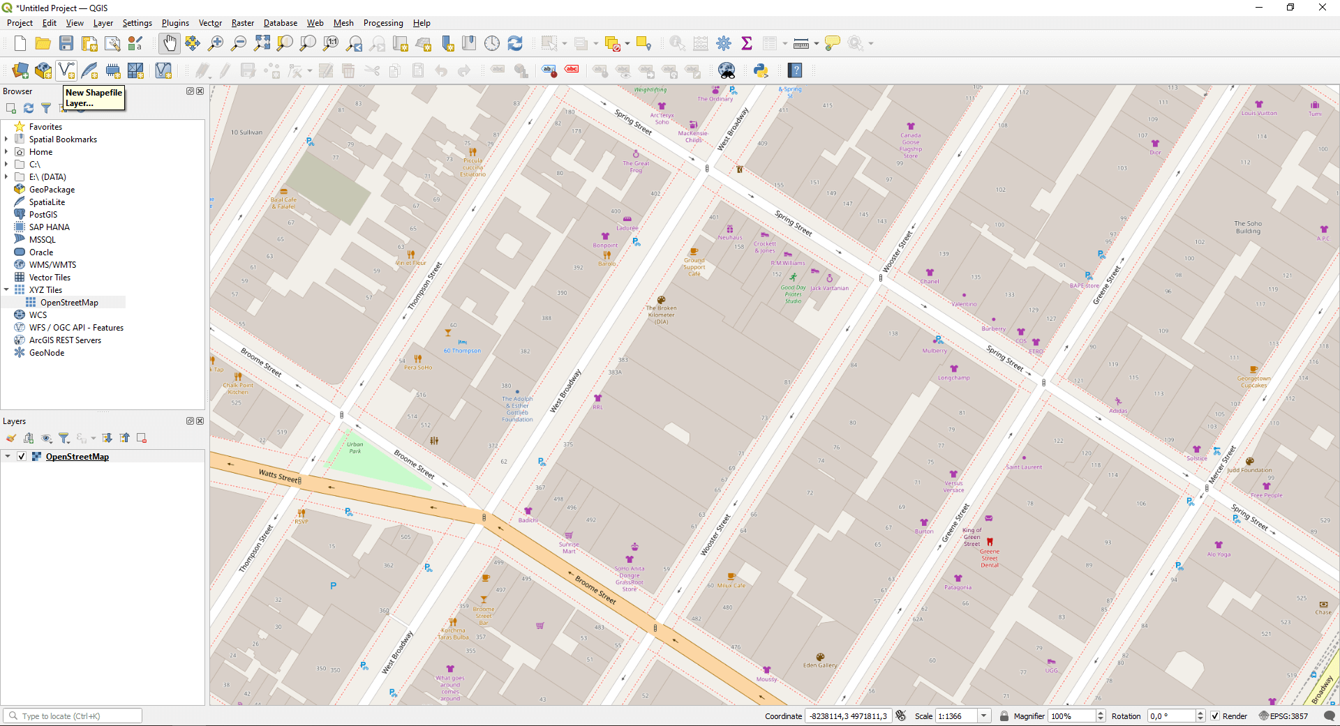
Zoom to an arbitrary area using the mouse scroll. We will vectorize a building chosen by you. Click on the third button on the menu bar above the map canvas which is “New Shapefile Layer…”. Can you figure out the next step? Yes, the name of the subtitle becomes reality, and we will create a shapefile. 

First you need to give the name and the location of the new file. It’s recommended to create a new folder for that operation because the software creates some additional files while creating the shapefile. At “file decoding” you can set the character encoding of the attribute table (which is actually the data content behind the geometry). If you are uncertain which one to choose then set UTF-8 encoding. This contains almost everything. The next one is the geometry type field.

Let’s take a little break here… Shapefiles, unlike CAD (DXF and DWG) type spaghetti models, are made up topologically. Okay, don’t close the blog yet, I will explain this, then we get back to QGIS. The essence of the spaghetti model is that points, lines and polygons can be in the same data table regardless of what object we want to display. In contrast, when working with a topological data model we need to determine in advance, what type of geometry we want to store in a data table. And that’s it, let’s get back to QGIS.

Let’s pick the “Polygon” option. When choosing dimensions, if we select the “Z (+M values)” option then we create an area that can be interpreted in 3D. Let’s make it exciting and select it! The next step is to set the coordinate system of geospatial data. Choose the 3857 Pseudo-Mercator. Here comes another interesting part that technically differentiates GIS from CAD. This is the attribute data table. Name a column (for example “building”) then beneath the “Type” field you can give the data type of the new fields. In this particular case  we use “Text” which is a simple string. Click on “OK” and now you can see that the shapefile has been added to the layer tree of the map. Select the new layer on the menu bar then click on the pencil icon to start editor mode.

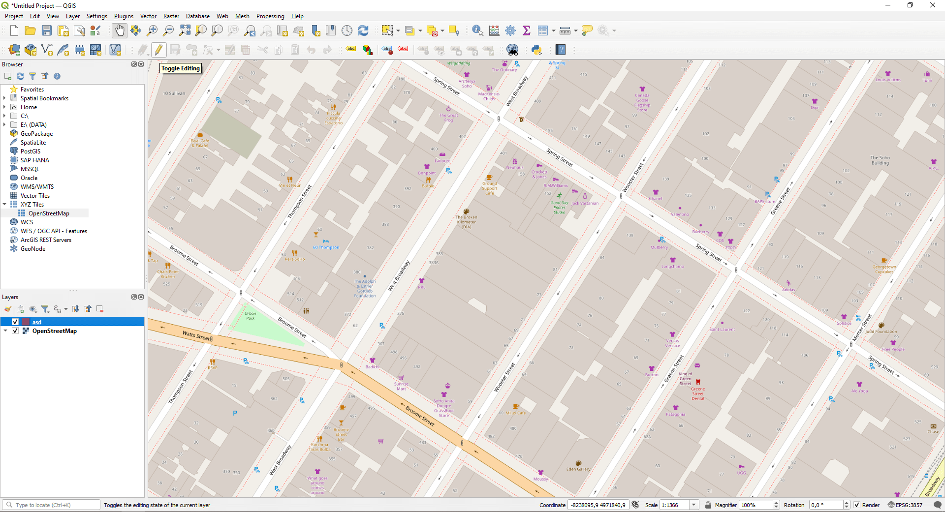
Afterwards you can pick “Add Polygon Feature” to activate the drawing. With clicking on the map, you can create vertices and between them an area appears. If you feel like you’re ready and your polygon covers the foundation of the selected building, right-click on the map to close the geometry. A small dialog box will appear to ask for attributes. Enter the data and click on “OK”. 

From the menu bar let’s pick “Vertex Tool ”. With that we can assign Z values to coordinates. The easiest way to do that is to press and hold the left mouse button and select your whole geometry. Then move your cursor above a vertex and press the right mouse button. A table will appear on the left.

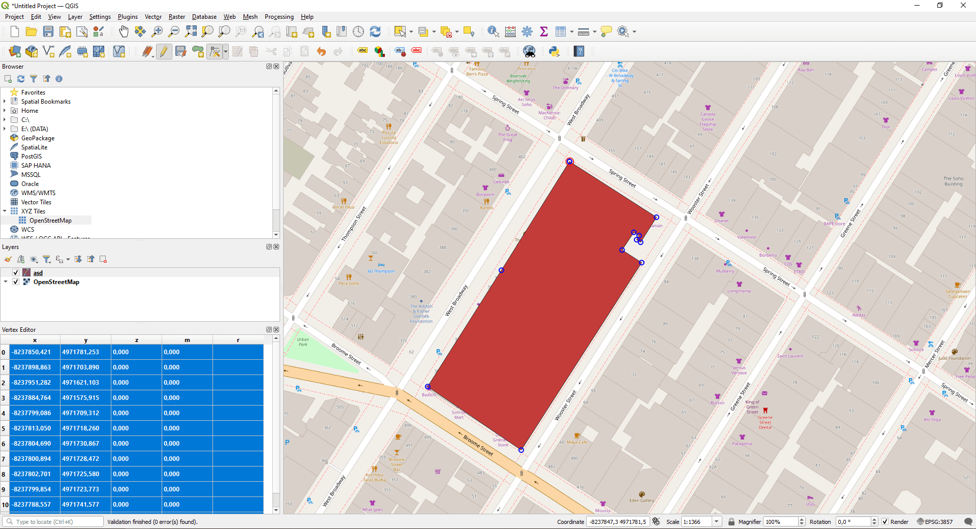
Change “z” values. Save the shapefile by clicking “Save Layer Edits” on the menu bar. Turn off the Editor mode and we are ready.

3D modeling using CG

In this chapter I will show you the 3D editing possibilities of the previously presented shapefile in Computer Graphics (CG) environment.

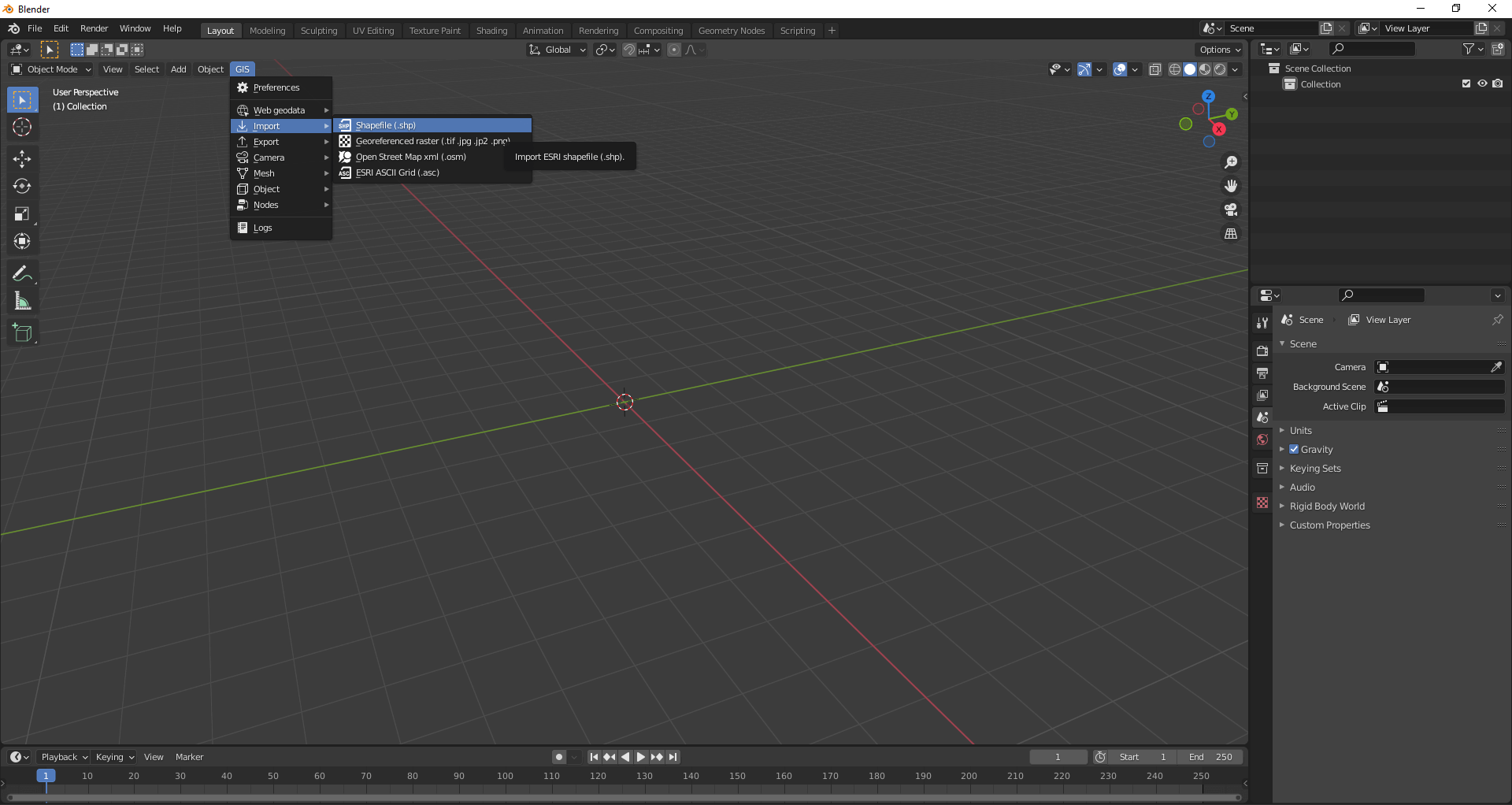
If you would like to try this technique you will need Blender and also BlenderGIS. Don’t worry, I’m not trying to sell anything, these are free open-source software.

After installing Blender and its addon, let’s start it. In the 3D model space, a small window will appear which disappears if you click outside of it. In the model space you see a small cube, a light source, and a camera. In this tutorial we don’t need them, so we delete all of them. Press “A” on your keyboard to select all the items then press “Delete” to delete the objects. Now the track (i.e. the model space) is all clear, let’s import the shapefile.

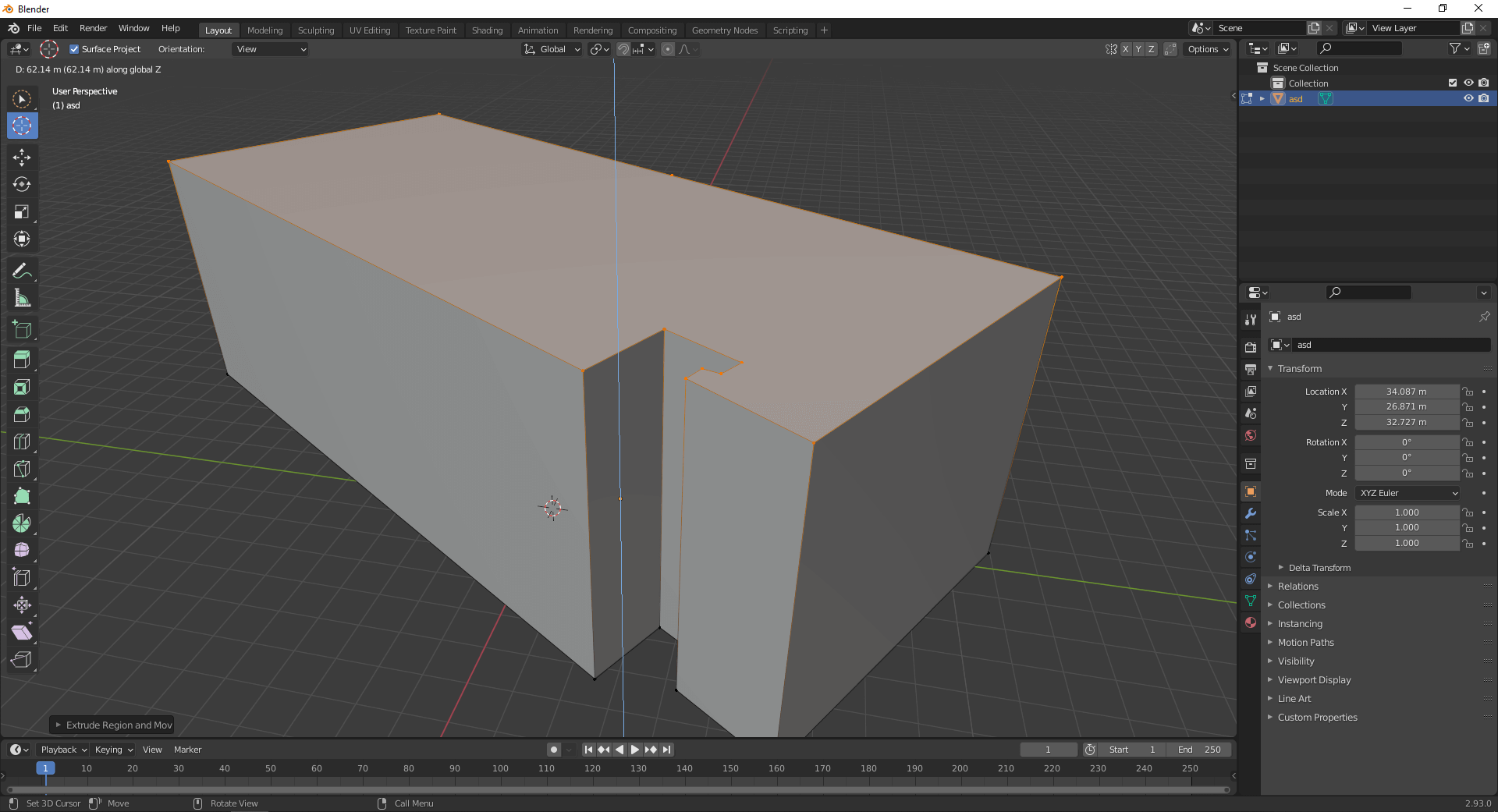
To edit, first select the geometry with the left click. Press the “Tab” key and now you are in editor mode. By pressing “A” again, you select all the vertices. Let’s extrude this area along the Z axis! Press the “E” key then move the cursor in the model space. It’s cool, isn’t it? 🙂

Save our 3D model. For that first exit editor mode by pressing “Tab”. Then export the model in OBJ format.

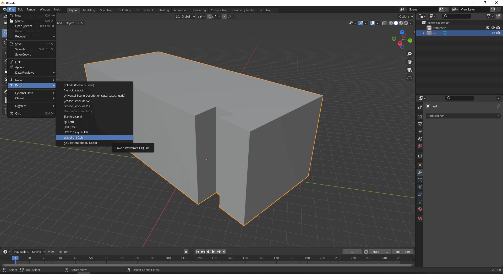
While exporting, take care of the following: on the right in the “Transform” menu set “Forward” value to “X Forward” and “Up” value to “Z Up”.
With the basic functions of Blender you can even create buildings and add texture to them. So if you want to unite GIS with 3D modeling, this software will be your best friend. Blender itself has a tremendous number of tools that will not be discussed in this introductory article. If you want to become a master of Blender, I recommend this YouTube channel. The guy is a genius.
If you are looking into the opportunities specifically in BlenderGIS and 3D modeling functions I recommend these videos.

Three Step Over Point clouds

In this section, I will present another software and multiple useful methods. For this I will use previously presented results.

If you want to complete the tutorial you will need another free software as usual. This is CloudCompare.
Sidenote: It’s possible that your antivirus will detect it as a dangerous software. If you feel uncomfortable installing it, just skip this, you can follow the steps presented here without having CloudCompare. But I’ve been using it for years now and it never caused any trouble. 🙂

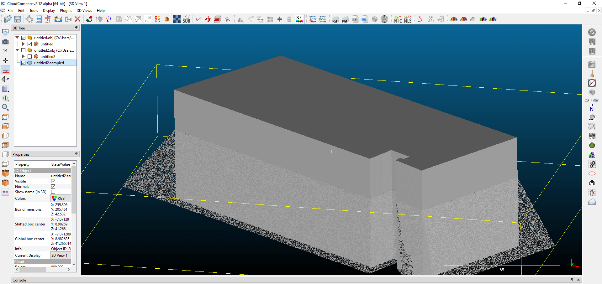
After starting CloudCompare, open the OBJ file made before. The software has the advantage that it can open and export a lot of file formats. 

To be honest with you I must admit I cheated, because I made a model in Blender which is a bit different from the one presented. I’ve done that to be able to make a comparison between the two models.

If you select the (mesh) layer of the 3D model in the menu bar above, then you select “Sample points on a mesh”, you can create a point cloud from the mesh. Here you can set the number of the points (for example: 100 thousand), the density, and also colors you want from your mesh model to inherit. After running, a new layer appears.

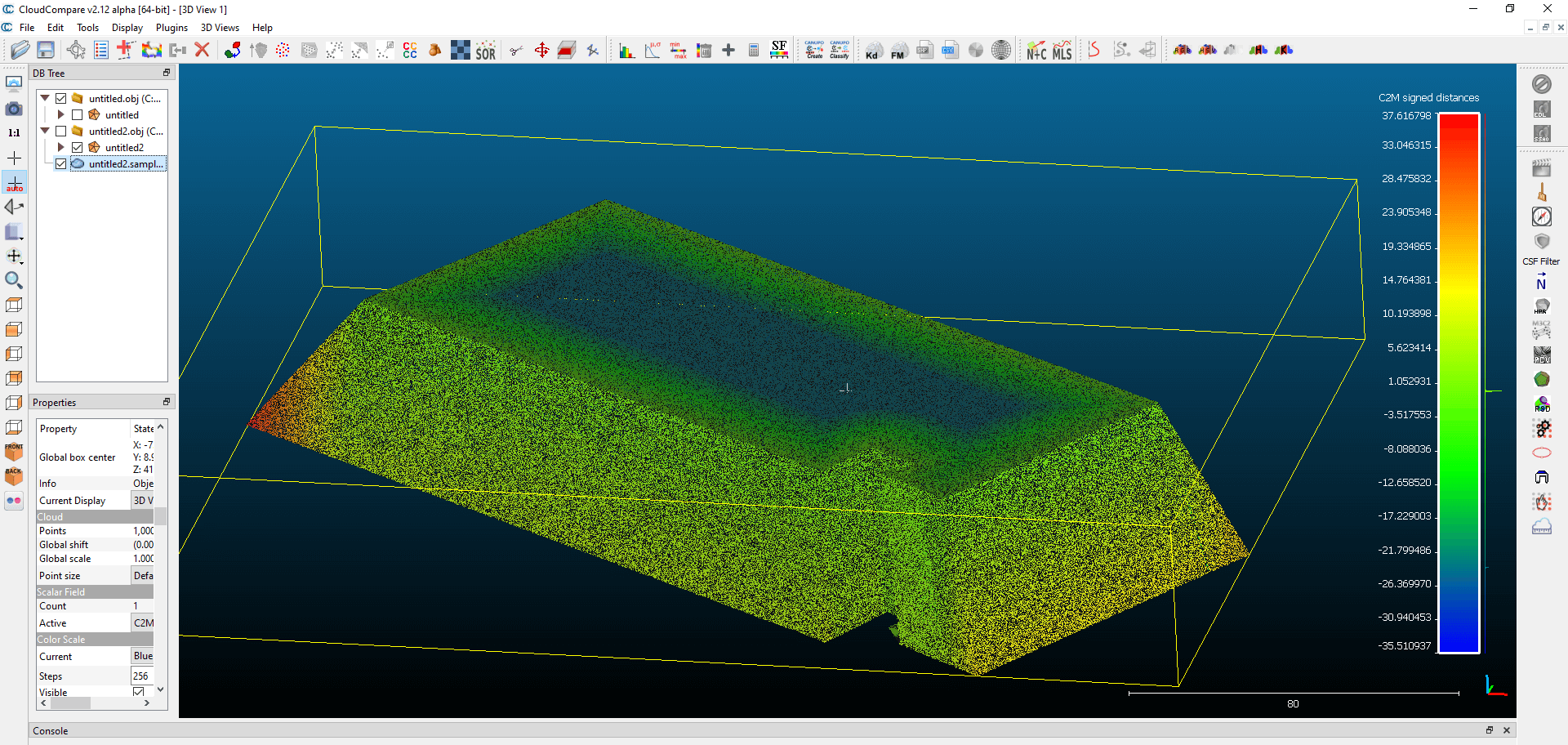
We will examine the differences and the distances between the point cloud and the mesh model. You can do that by holding “Ctrl” button and selecting the new point cloud layer and also the mesh layer. Then  select “Compute cloud/mesh distance” on the menu bar. If the process was successful, you can examine the extent of difference on a scale from red to blue. Red areas indicate positive distance, while blue areas indicate negative distance.

Apart from these, CloudCompare is a great tool to calculate the volume of the object. It is also possible to compute using UAV or ground photogrammetric and even LiDAR point clouds. You can read more about that in a later article.

Raster geospatial data

In this chapter we will discuss how to create a DEM without photogrammetrical or LiDAR based output. I will show you how to easily create a slope and an aspect map by using a DEM file. This is going to be exciting so don’t give up just yet. 🙂

Creating DEM from vector

So if you are into photogrammetry and LiDAR technology, creating a DEM won’t be a novelty. However you can also create a digital elevation model in QGIS using GPS points or contour lines. 

In this example we will create a DEM from existing contour lines. If you are curious how to make a contour line map from an old paper map, read this article (). 

As shown before, open the shapefile in QGIS.

We can make a raster terrain model with the help of interpolation.Interpolation is a difficult geostatistical tool that can predict values of the areas with lack of data, based on the known points. The most common interpolation tools are Inverse Distance Weighting (IDW), Spline, Kriging. All of them are available in QGIS. I need to highlight that geostatistical calculations can only be used if the shapefile’s attribute table contains the elevation, or the vertices of lines have “z” coordinates. 

First we need to find the processing toolbox. For that, in QGIS you right click on the top menu bar and choose the “Processing Toolbox Panel” option, then tick it.

After all this, a search bar on the right side appears. Type “IDW” and choose the first option. Now you see a new window which can seem a bit complicated. Here you can pick which field you want to examine with the geostatistical tool. Resolution and geospatial extent also need to be set. 

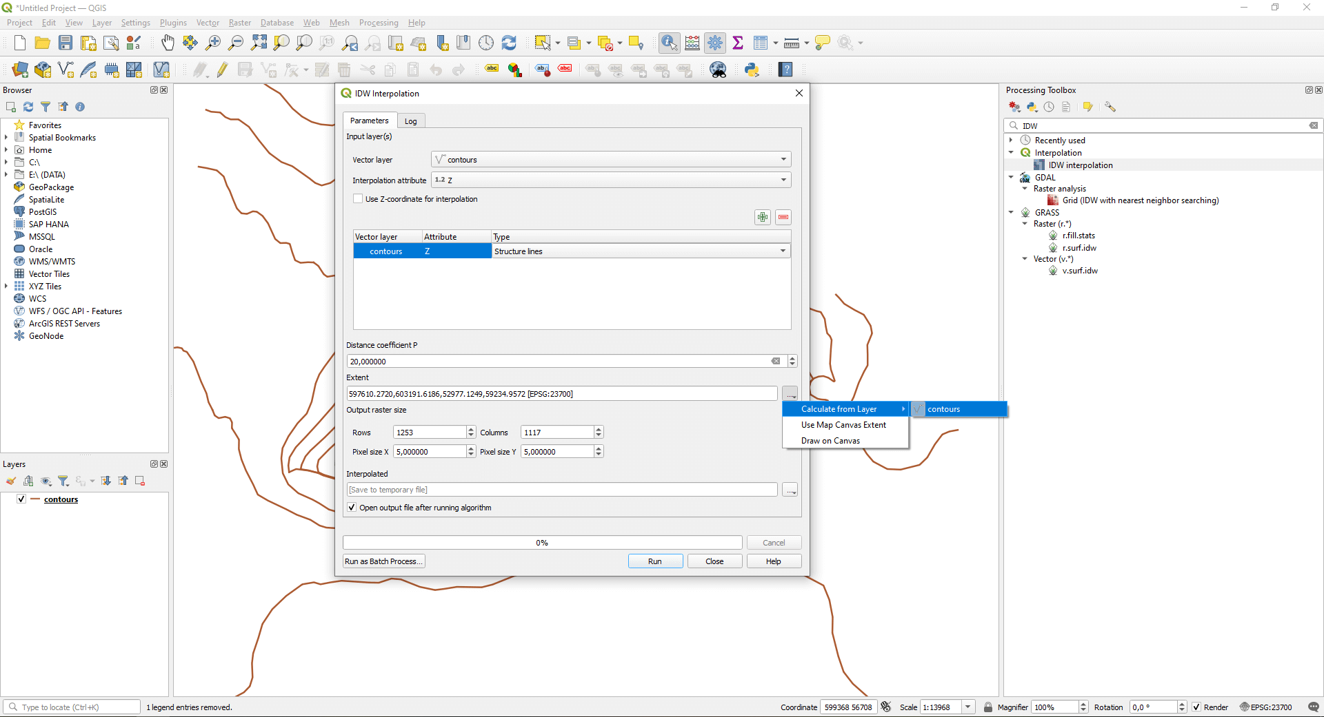
Click on “Run” and the calculation begins. This process can take a few minutes depending on the size and resolution. 

Thematic content

Let’s see what we can make with a raster, actually a DEM, to be precise. In this chapter we will make a slope- and aspect map. Now we need to search for the word “slope” in the well-known processing toolbar of QGIS. We run the function with default settings by choosing the first option. The result will be a nice black-white map, but we can style it. We double-click on “Slope” layer, then in the “Symbology” menu change “Render type” to “Singleband pseudocolor” value. Pick an arbitrary “Color ramp” then press “OK”. 

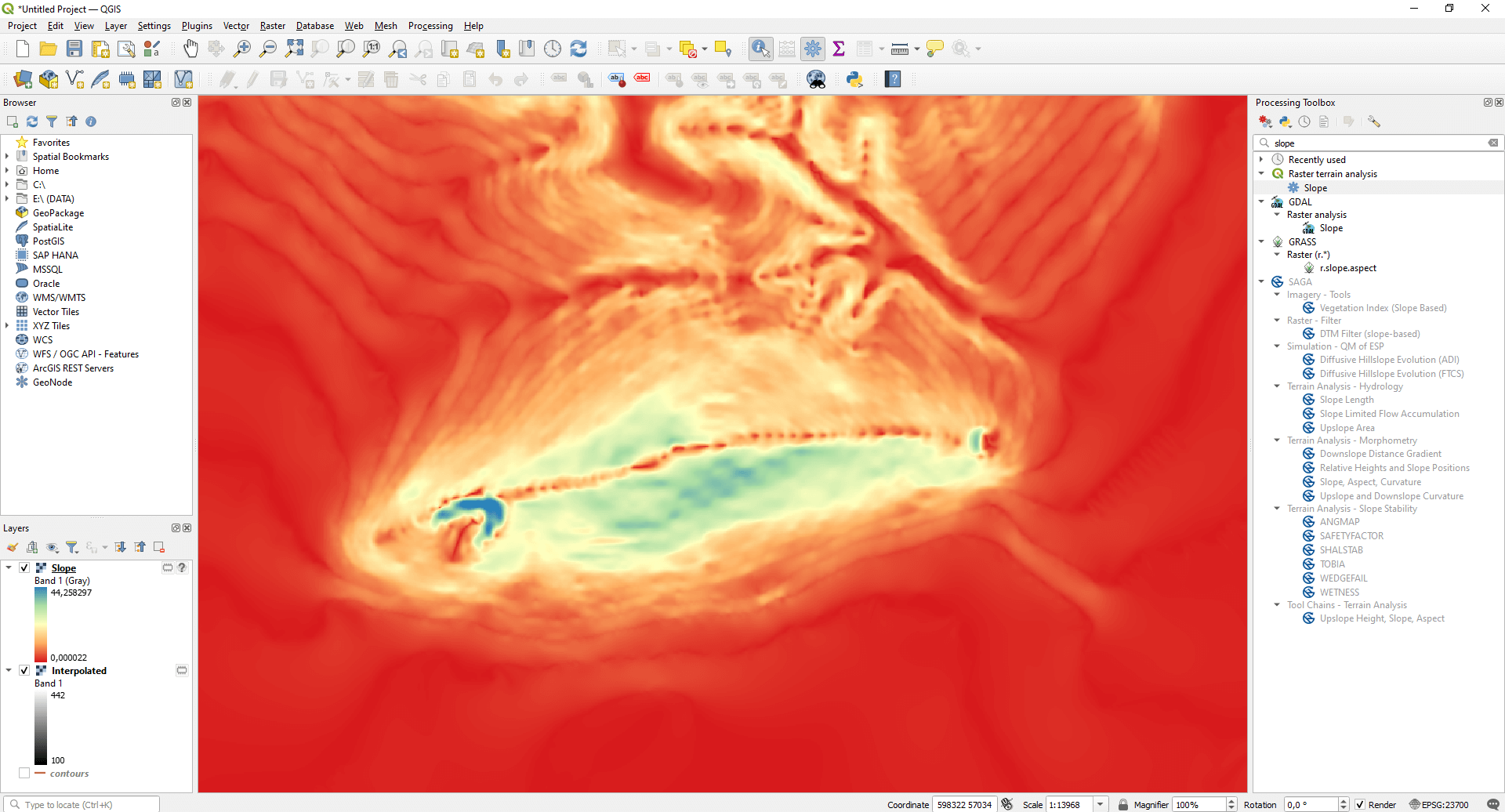
Now on the map you can see the slope angles of the surface with categorized coloring. Of course, these maps can be created for roofs and for buildings too. 

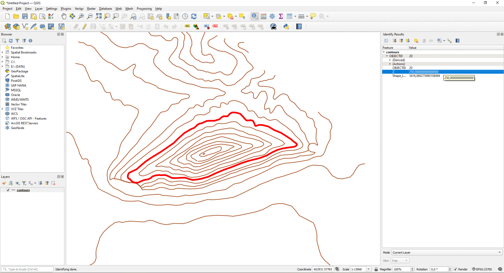
In the search field we type “aspect” and run it on the DEM with default settings. The result will be indistinct, but you can set coloring based on directions in the “Symbology” menu. You can see that in the following picture:

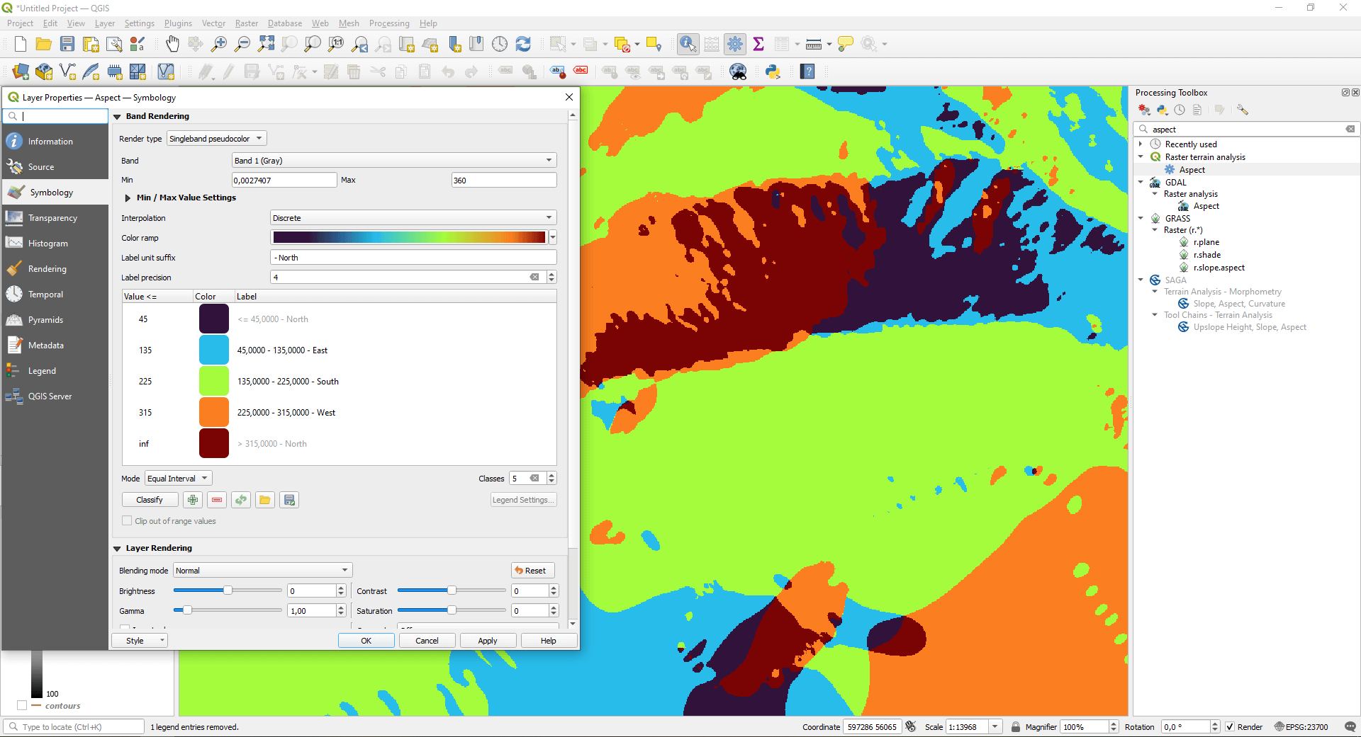
Based on all these, we can define which areas get more sunlight (also for larger areas). This is important in an agricultural aspect but also important when installing solar panels. 

Fields of use of Geospatial data

In this last chapter I’ve collected the most important fields where geospatial data can be used (of course in a non-exhaustive list).

Geospatial data give opportunities to inspect agricultural and forestry tasks from a different angle.

• Investigation of the health of vegetation becomes possible via mass data collection methods. This can result in a more accurate yield estimation.
• Multispectral cameras allow us to early diagnose and map tree diseases
• Wildlife damage can be measured and mapped in a larger area 
• We can make up to date maps of drought damage
• It’s also possible to regularly survey forest roads and hiking trails We can create high accuracy soil maps with extensive attribute data

In the construction industry CAD and BIM based geospatial data is becoming dominant nowadays. These technologies allow us to represent whole buildings as 3D models, including wires and pipelines together.

3D models and aerial maps are also importantly related to archeological research and monument protection. Investigation of layouts from old buildings or restoration of monuments for instance (before and after).

Today, raw material research is also based on satellite and UAV images. Searching for natural resources like oil and other mineral treasures is a field where remote sensing (and geospatial data) is widely used.

And let’s not forget that city councils and other government agencies can control their cities via geospatial data. When I say that I mean SmartCity projects which are based on geospatial data.

Media- and entertainment industry, insurance sector, the law, real estate market, disaster management and of course transportation are sectors that have started to adopt technologies based on geoinformatics.

I hope this article successfully describes geospatial data and how you can use them even with free software. Even though here we only had a few examples, in our other articles we discuss these topics in more detail.

Did you like what you read? Do you want to read similar ones?

If you really like what you just read, you can share it with your friends via our social media sites.