UAV and GIS encounter: Where to build a lookout or radio tower?

It is common to present the data analysis potential of GIS by filtering the optimal spatial parts. Our current article will be about this, so we’ll look at which points within a given area, according to certain criteria, are appropriate for building a lookout or radio tower. 

How are drones connected to this? GIS software without data are one-legged giants! The basic data for GIS (e.g., DEM, settlement boundary or road network map) can be created by aerial surveying. If you are interested in how to create a vector road network or settlement boundary map from an orthophoto, read our previous article.

We determined the following criteria for selecting the optimal location for the lookout / radio tower:

1. It’s important to place the tower high enough, so the highest point of the area, and those areas that are 150m lower can be optimal.
2. Choose a location that is at least 500m away from any settlements so as not to disturb the residents.
3. Take care that the chosen position should not be further than 100m from the road network to make it easily accessible by car.
4. The radio/lookout tower will be 15m high.
5. From the available locations, select the point with the largest area of view (15 meters above the current terrain). This is important because if we are talking about a lookout, we want to show visitors as much field as possible, if we are talking about a radio tower, we need to have as high signal strength as possible. 

Sidenote: We’ve done the process in the newest QGIS Desktop 3.24.0 software. If you’re using older versions then I draw your attention that the techniques described here will only work with QGIS 3.x versions. Also, if the version with GRASS GIS functions starts separately (e.g., QGIS Desktop 3.14.0 with GRASS 7.8.3), start the version with GRASS functions. The new QGIS software already includes GRASS functions by default.

FILTERING THE HIGHEST POINTS IN GIS

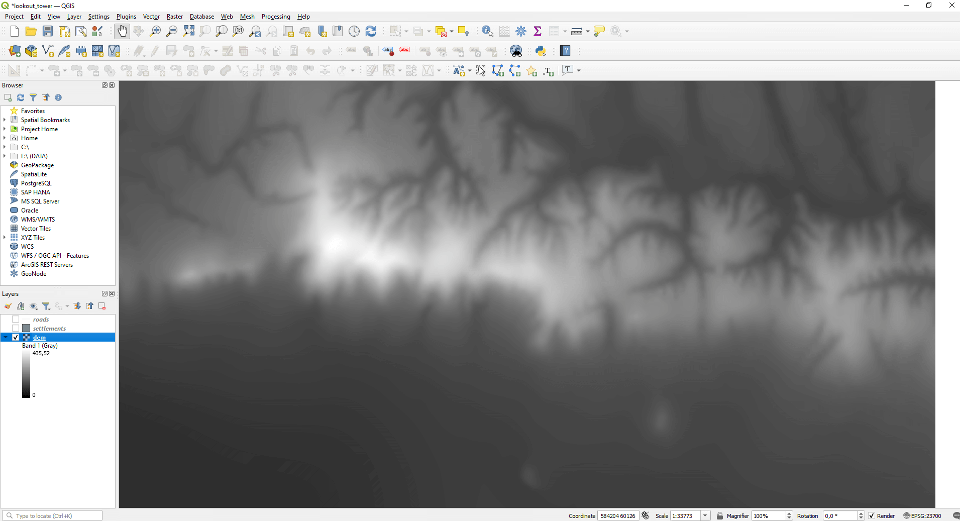
In order to be able to select the highest point of the area, and those areas that are 150m lower, we will need a DEM. If we open the terrain model under QGIS, then the height value of the highest point becomes visible in the layer tree.

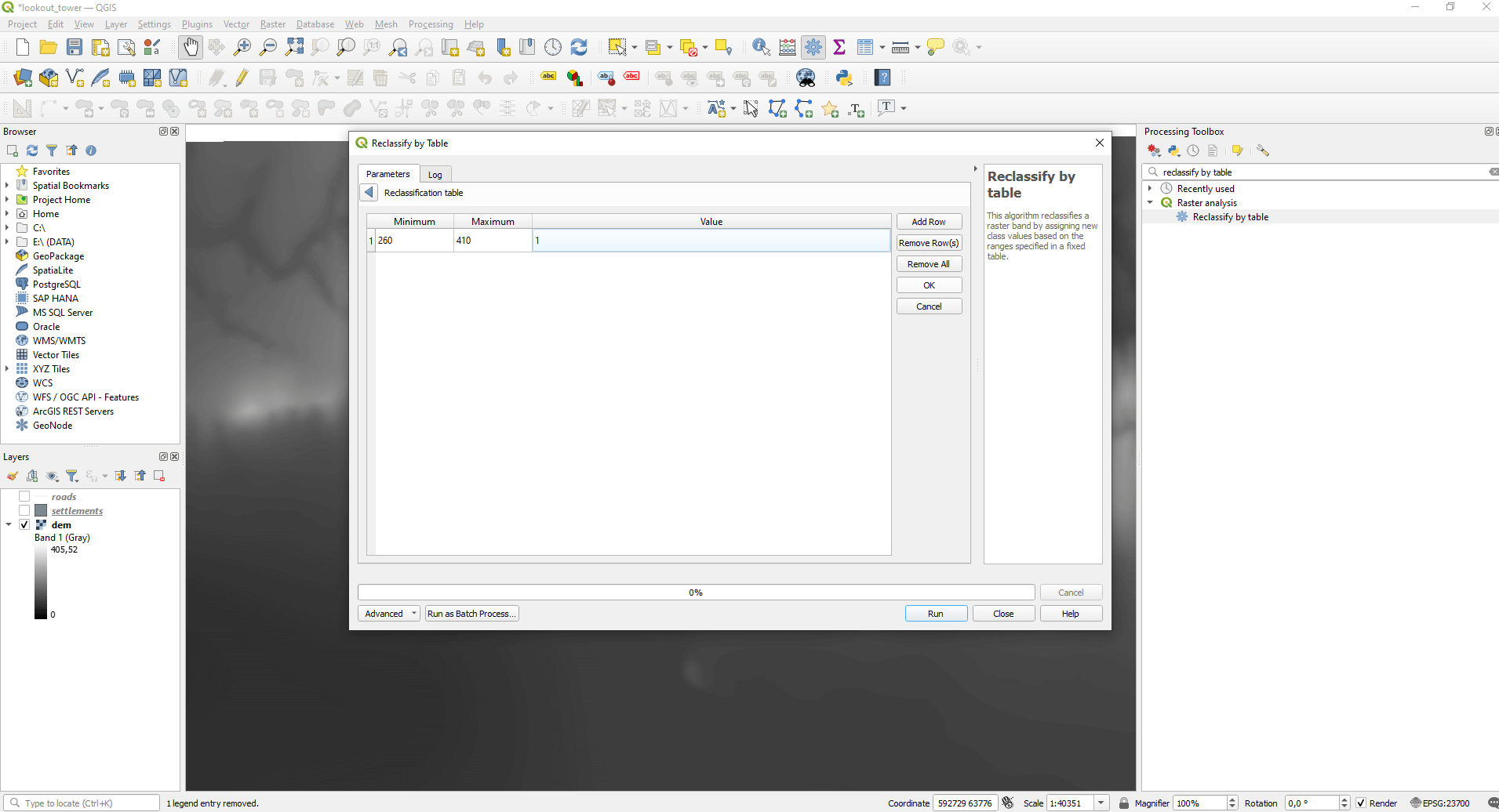
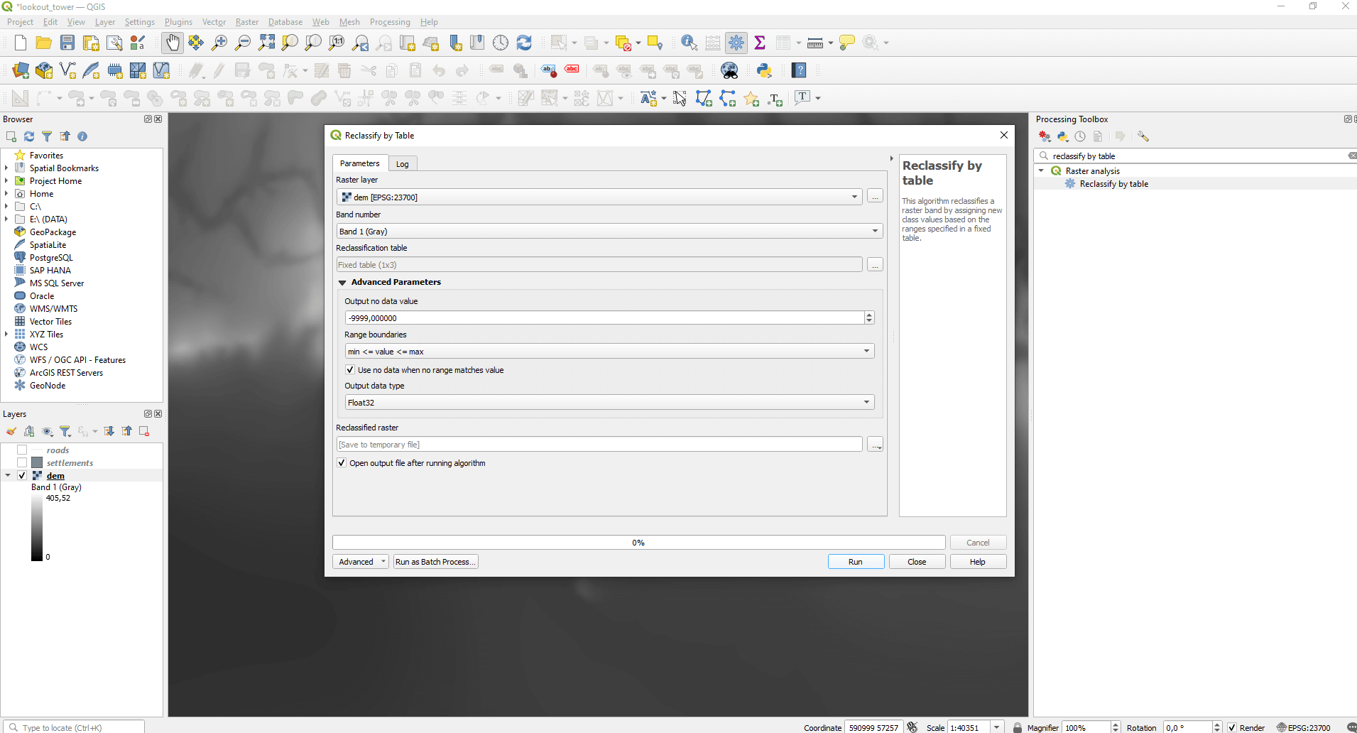
The “Reclassify by Table” function can be found under “Processing Toolbox”. By opening this, the DEM layer must be selected, and within this you can set the range of height values under the “Reclassification table” option. In my example, I set “Value” to 1. All you have to do is set the raster value to 1 in the cells you are looking for, you get all the other “NoData” values.

I recommend turning on the “Use no data when no range matches value” option. In the following image, you can see with what settings I ran the function. 

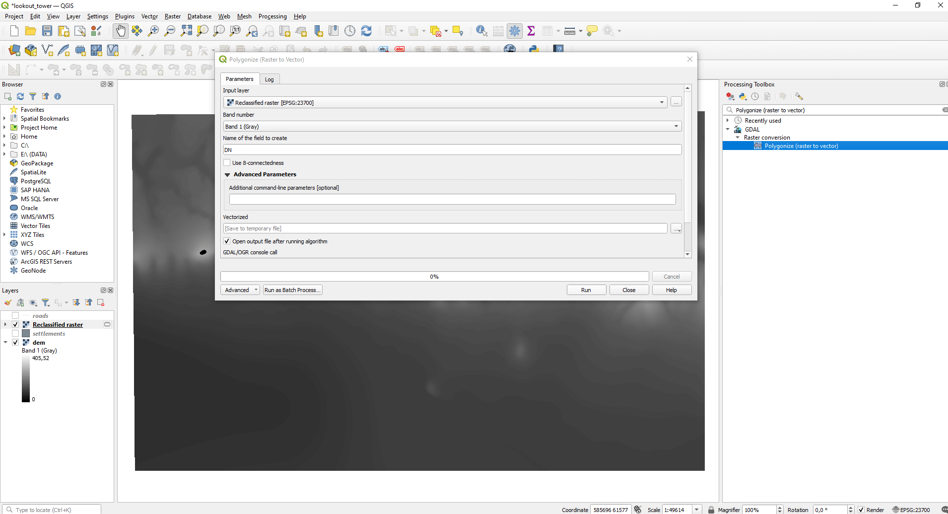
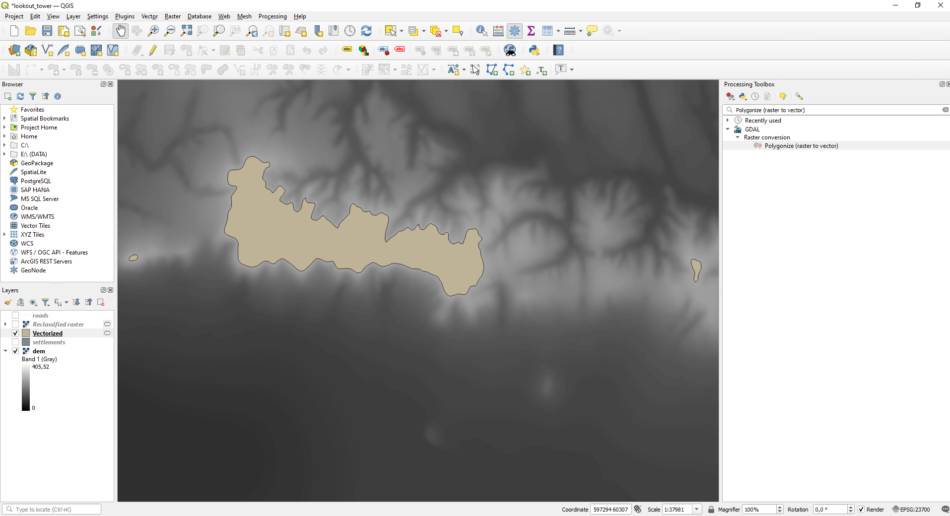
If everything went as planned, a black blob will appear on the map. This is a raster file; in the following steps we will work with vectors. There are some cases when it’s easier to work with a unified data model and I think this is also such a case. Convert the selected area into a vector. In the “Processing Toolbox” search panel, type “Polygonize (raster to vector)”. Open the popped up GDAL function and select the previously generated raster in the “Input layer” field. 

The result is a vector file that fits well with the boundaries of the raster.

FILTERING THE AREA OF THE SETTLEMENTS

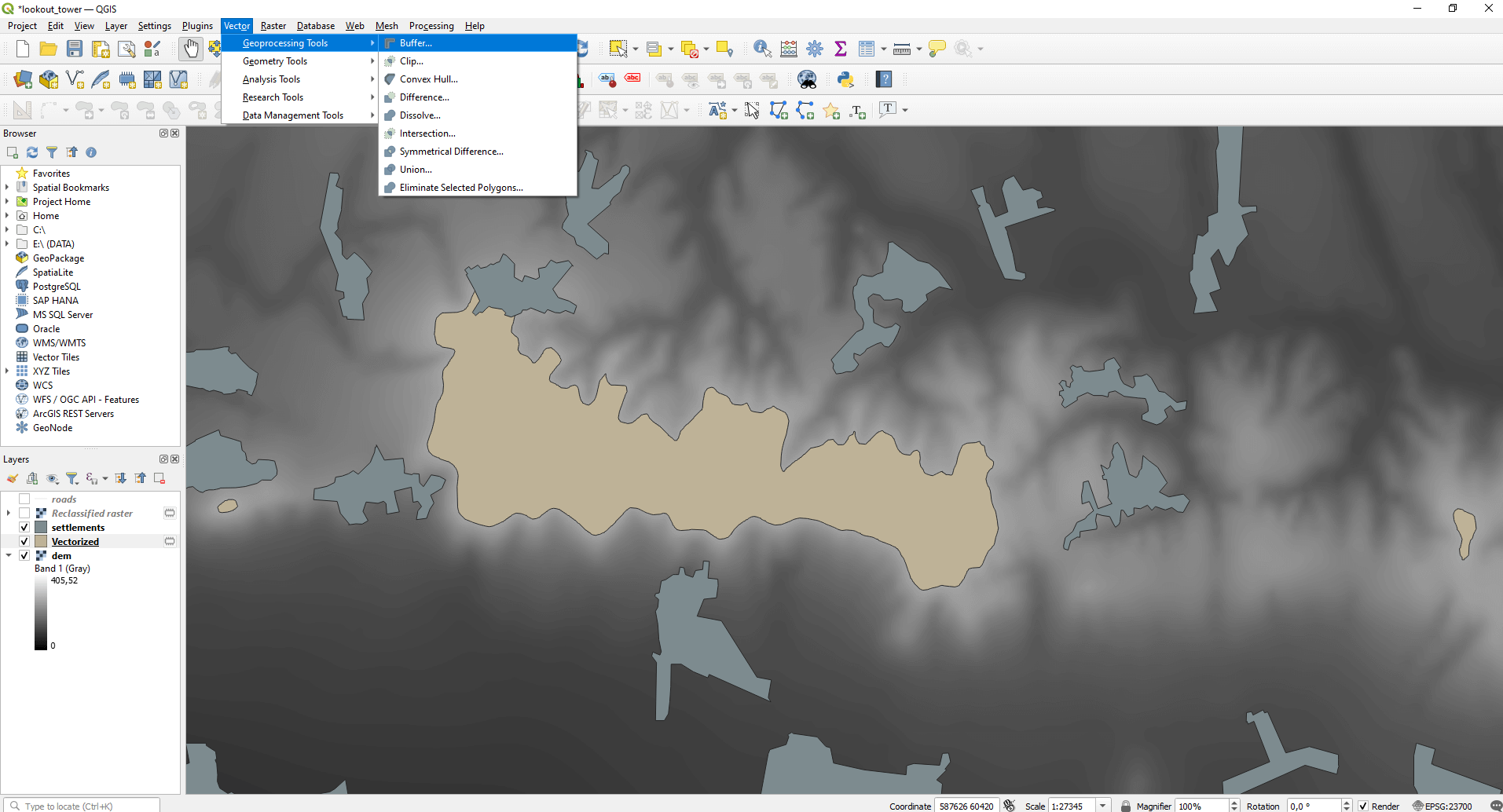
According to the criterion, a 500-meter zone of settlements must be created and then these areas must be removed from the potential areas. If we do this, the remaining places will fall farther from the populated zones than 500 meters  (as the crow flies). First, open the vector layer of settlements. Then, a zone around each object can be generated with the “Vector / Geoprocessing Tools / Buffer…” function in the top menu bar.

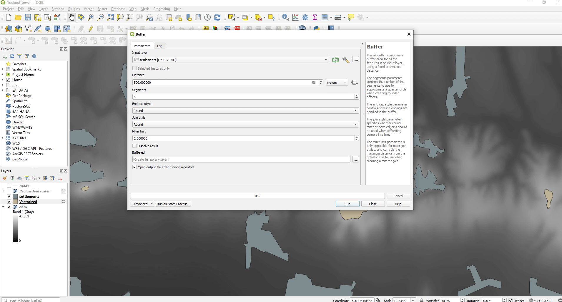
Choose the settlement’s vector layer, then set a distance of 500 meters.

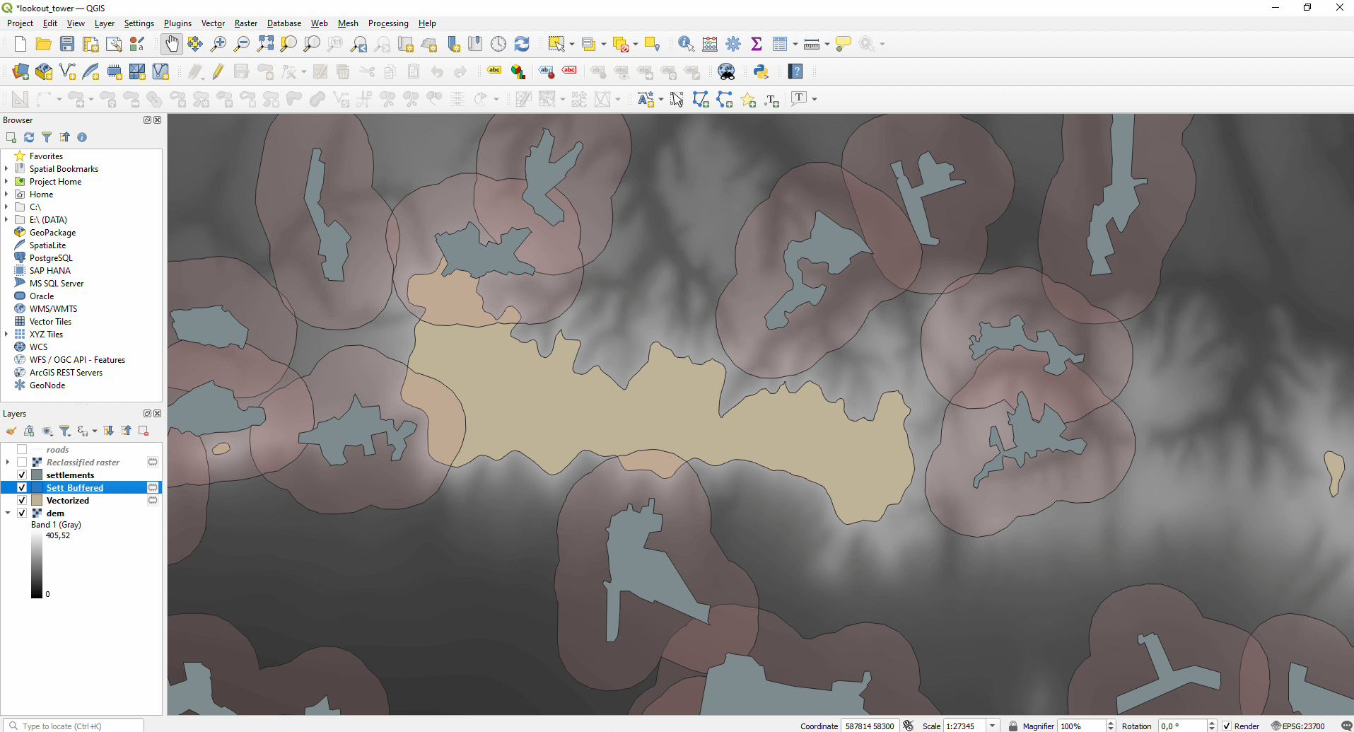
The result is as if obese settlements were scattered on the map. ☺ There are several areas that overlap with the hilly locations selected in the previous chapter.

We need to delete the overlapping areas because they don’t meet our criteria system. The easiest way to cut out unsuitable areas is to use the “Vector / Geoprocessing Tools / Difference…” function.

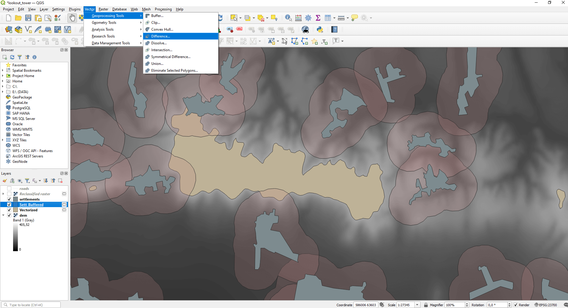
Here, enter the vector altitude-optimal locations at the “Input layer” and then the settlements with the extended zone for the “Overlay layer”.

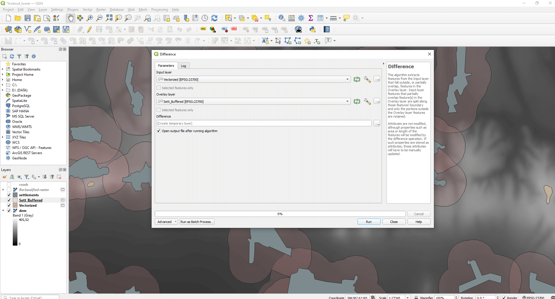
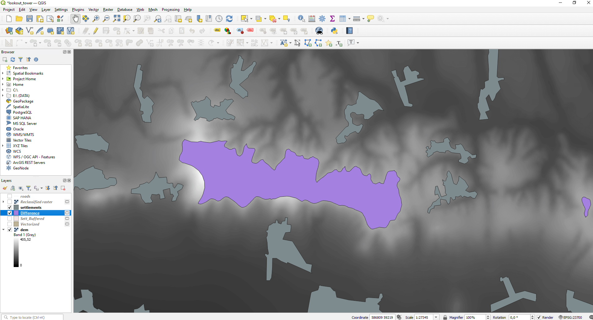
The size of the optimal area has been reduced with the new partial result.

DESIGNATION OF THE AREA NEARBY THE ROAD NETWORK IN GIS

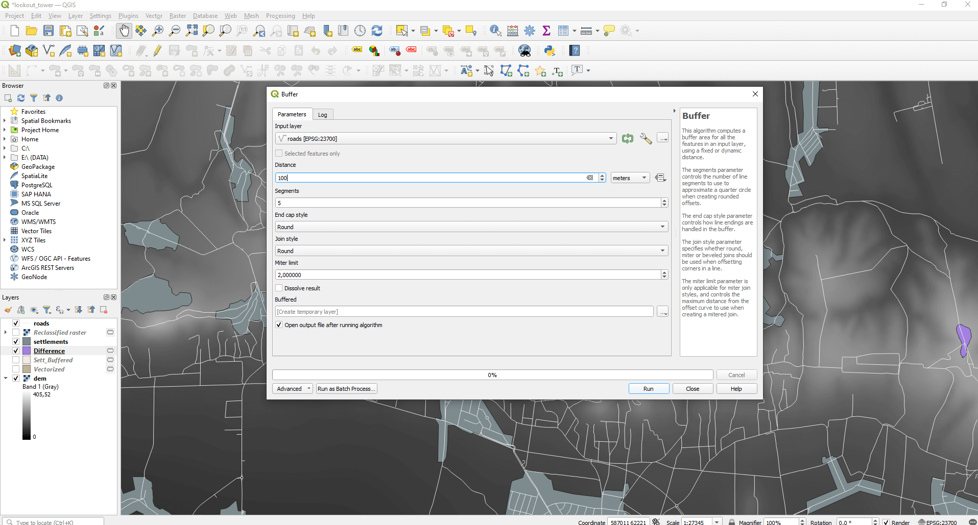
In this chapter we filtering the areas according to the third criterion. This means we need to select areas that are 100 meters from the road network. We create the 100 meter zone of the road network layer using the “Buffer” function.

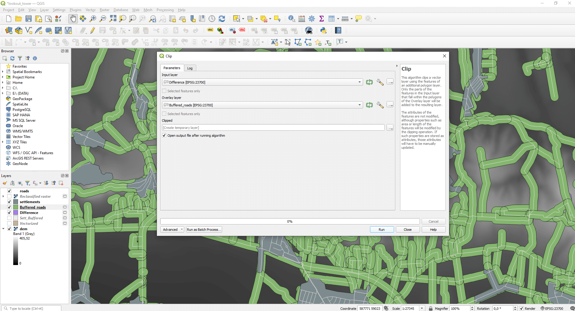
The result is like a worm map. I wonder…is there a map showing earthworm varieties…? 🙂 In contrast to the previous operation which required deletion, we are interested in common points here, so we use the “Vector / Geoprocessing Tools / Clip…” function.

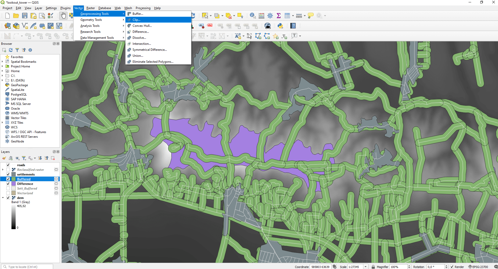
You can imagine how the “Clip” works as we have a dough (the area sorted out in the previous chapter) and we have a dough form (road network area). With the form, we want to extract the relevant areas because these will be valuable for us. Therefore, the “Input layer”, which we want to extract from is the “Difference”, the result of the previous chapter. While the “Overlay layer” is the shape with which we want to extract, so it’s the area of the road network.

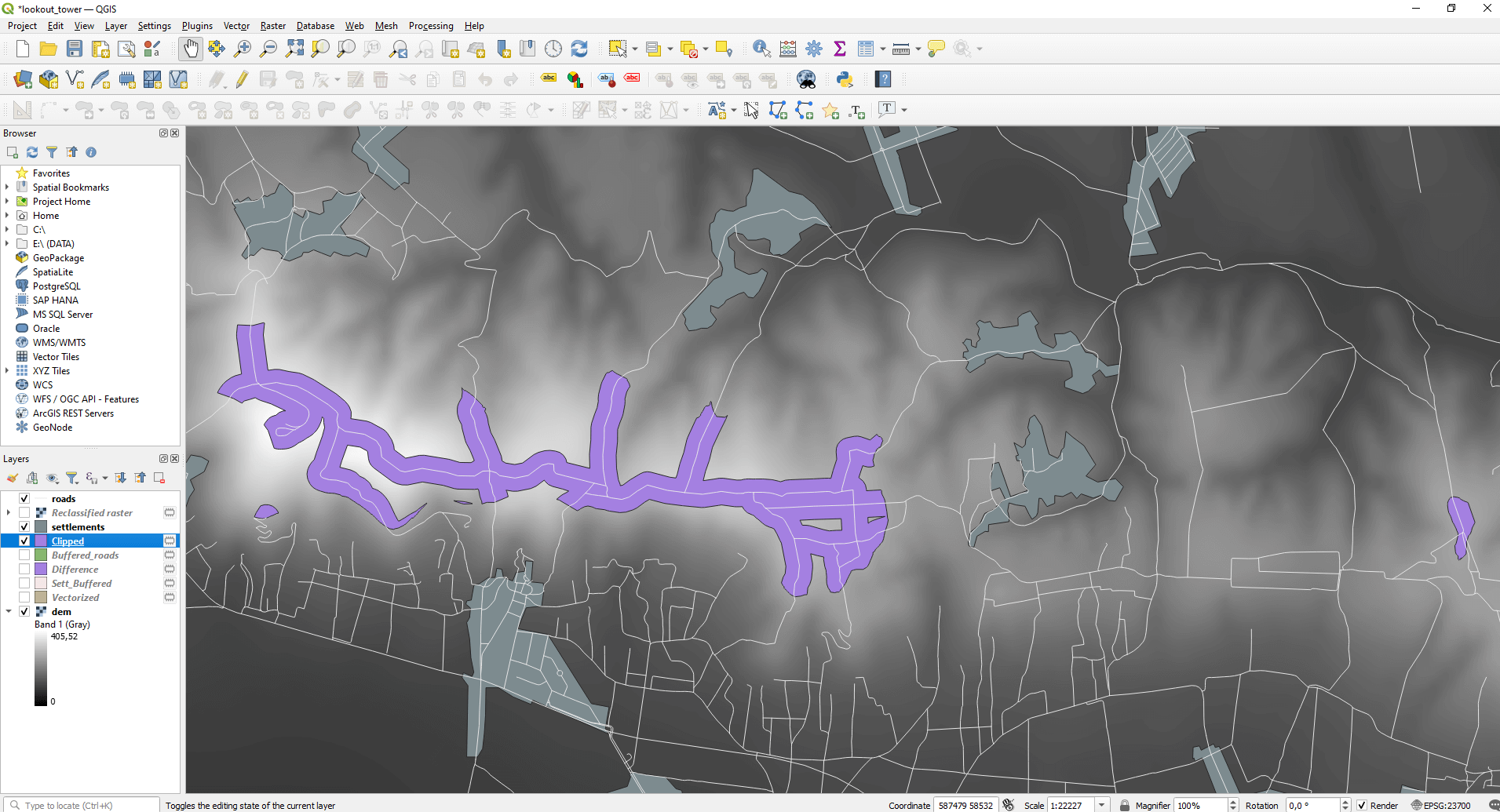
The result shows that we have further narrowed down the appropriate places.

THE AREA OF VIEWSHED ANALYSIS

To analyze the viewshed, there are two functions in QGIS: GRASS and GDAL. Both functions can only calculate the viewshed with points, but we have a polygon here. This chapter will be a bit more complicated than the previous ones, as we get to our goal with solving several subtasks:

1. In the first step we need to fit points to the polygon
2. As a second step we run the “Viewshed” function on every possible point. Then we need to calculate the viewshed of every map in hectares.
3. Finally, the third step is to select the point which belongs to the largest area of the viewshed analysis.

It’s quite a challenge, so let’s approach the problem in steps.

ALLOCATION OF THE POINTS WITHIN THE OPTIMAL AREA

You can fit the points by selecting the “Vector/Research Tools/Random Points Inside Polygons” function. 

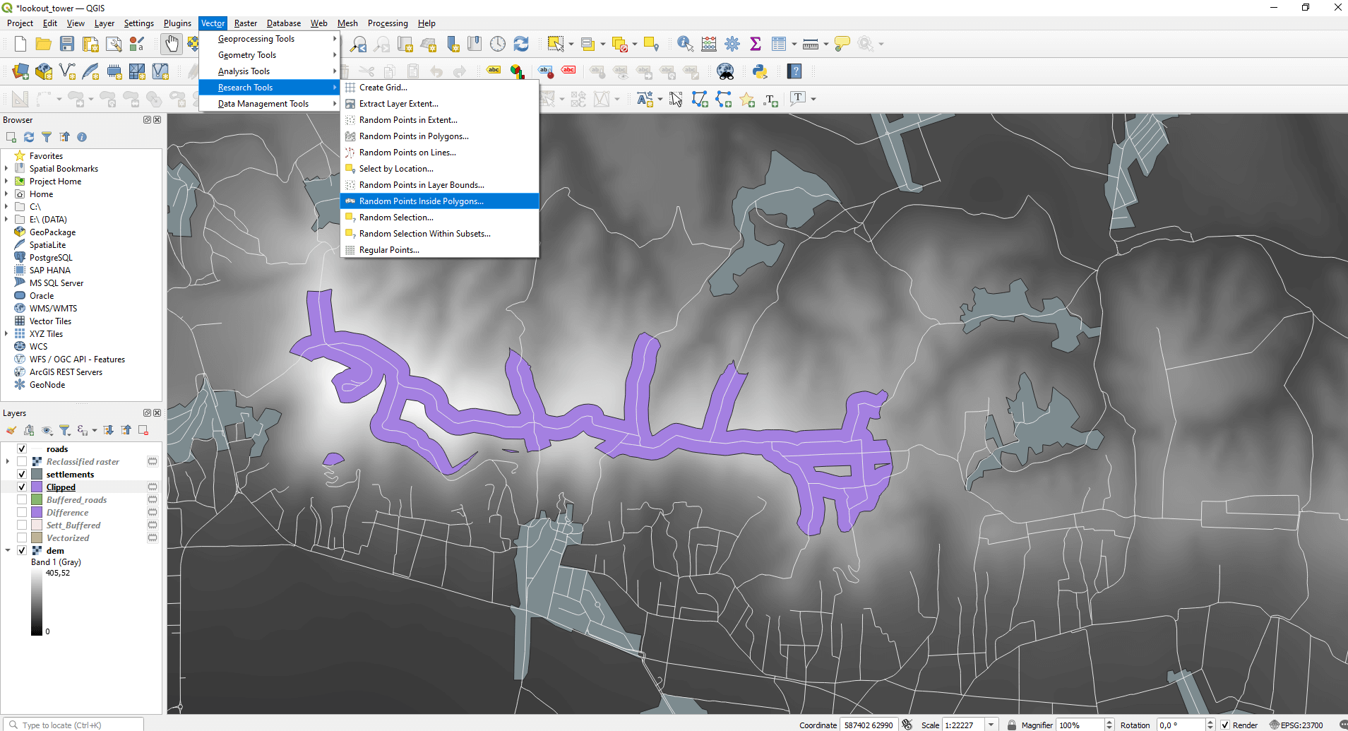
The function allows us to place points in a regular pattern within the specific area. For “Input layer”, select the filtered area (clipped) and set how many points you want to place within the area with the “Point count or density” function. It’s not a good idea to set an unrealistically high number here, as remember that separate maps must be created for each point too! I also set the “Minimum distance between points” to make the spatial distribution more even.

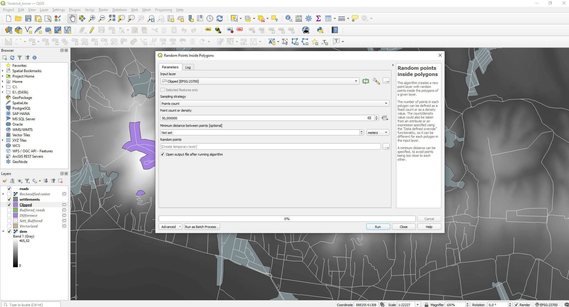
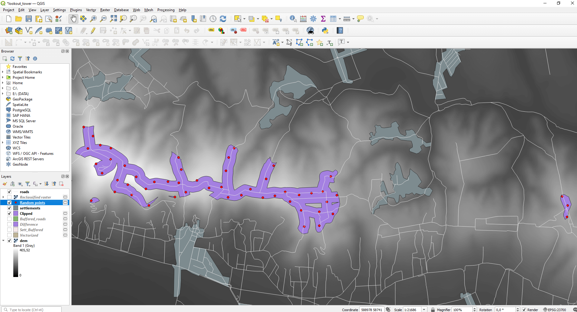
The result is a well-defined set of points with a regular pattern. Even though instead of the previously set 50 points QGIS generated 53 due to the distance setting.

GENERATING VIEWSHED MAP 

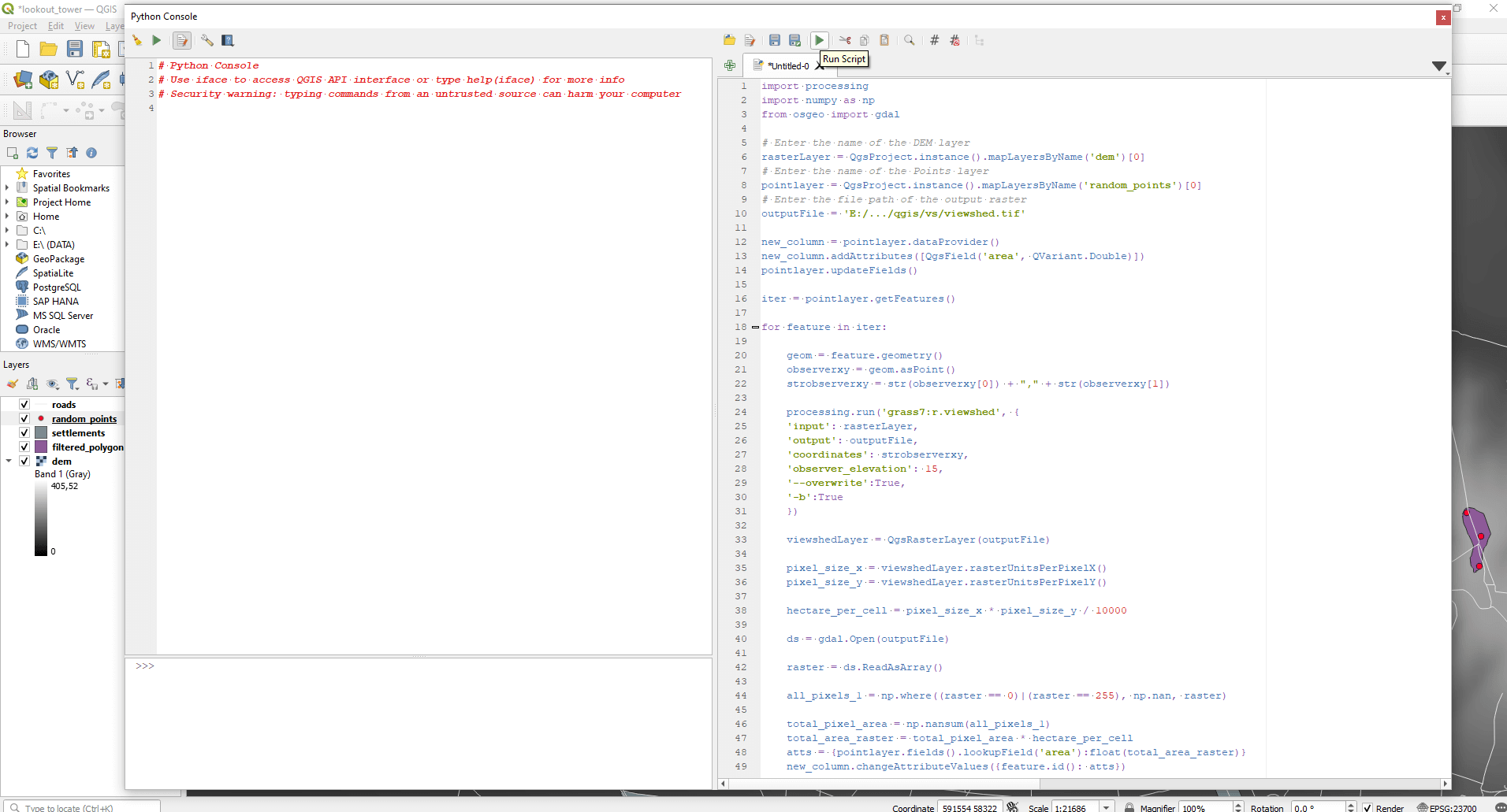
Probably generating the viewshed map causes the biggest problem. Just think about it. You need to run the “Viewshed” function for all the 53 points manually, then you need to calculate the area of the viewshed analysis. If this meant more potential locations or a higher sampling density, it would take up days with this. But not for us! A lazy person, like myself, learns to automate processes and let the computer work instead. In addition, the whole process becomes repeatable and controllable with the code. Let’s write some Python code that will do the dirty work for you! 🙂

In QGIS open the “Python Console” which is indicated with this icon: . Then press the “Show Editor” button. Copy the following code into the text area.

Sidenote: Before using the script, I share some important info. In the code I indicated (the texts after the # character) which variables you need to change. Take care to enter the path using „/” instead of „\”.
The other important thing is that I’ve written the code with the GRASS function. If you want to know more about this, you can read the detailed description here. I set the value of ‘observer elevation’ to 15 meters for this example. If you’re planning a lookout/radio tower with different parameters, simply change this value.

import processing
import numpy as np
from osgeo import gdal
 
# Enter the name of the DEM layer
rasterLayer = QgsProject.instance().mapLayersByName('dem')[0]
 
# Enter the name of the Points layer
pointlayer = QgsProject.instance().mapLayersByName('Random points')[0]
 
# Enter the file path of the output raster
outputFile = 'C:/Users/.../YOUR FOLDER/viewshed.tif'
 
new_column = pointlayer.dataProvider()
new_column.addAttributes([QgsField('area', QVariant.Double)])
pointlayer.updateFields()
 
iter = pointlayer.getFeatures()
 
for feature in iter:
 
    geom = feature.geometry()
    observerxy = geom.asPoint()
    strobserverxy = str(observerxy[0]) + "," + str(observerxy[1])
 
    processing.run('grass7:r.viewshed', {
    'input': rasterLayer,
    'output': outputFile,
    'coordinates': strobserverxy,
    'observer_elevation': 15,
    '--overwrite':True,
    '-b':True
    })
 
    viewshedLayer = QgsRasterLayer(outputFile)
    
    pixel_size_x = viewshedLayer.rasterUnitsPerPixelX()
    pixel_size_y = viewshedLayer.rasterUnitsPerPixelY()
 
    hectare_per_cell = pixel_size_x * pixel_size_y / 10000
 
    ds = gdal.Open(outputFile)
 
    raster = ds.ReadAsArray()
    
    all_pixels_1 = np.where((raster == 0)|(raster == 255), np.nan, raster)
    
    total_pixel_area = np.nansum(all_pixels_1)
    total_area_raster = total_pixel_area * hectare_per_cell
    atts = {pointlayer.fields().lookupField('area'):float(total_area_raster)}
    new_column.changeAttributeValues({feature.id(): atts})

After you’ve set everything, press the green triangle icon to run the script. Then feel free to go and have a coffee, you deserve it! 🙂 Isn’t is better when the computer works instead of you?

The presented code computes the viewshed map for every single point but always overwrites the output file. I’ve written it this way to be more space saving. If you’d need a data set which exports all the maps one by one, use the following code.

Sidenote: Compared to the sidenote for the previous script, you only need to make a small change in the code. At the end of the absolute path to save “viewshed” maps, do not type “.tif” after the file name!

import processing
import numpy as np
from osgeo import gdal
 
i = 0
 
# Enter the name of the DEM layer
rasterLayer = QgsProject.instance().mapLayersByName('dem')[0]
# Enter the name of the Points layer
pointlayer = QgsProject.instance().mapLayersByName('Random points')[0]
# Enter the file path of the output raster
outputFile = 'C:/Users/.../YOUR FOLDER/viewshed'
 
new_column = pointlayer.dataProvider()
new_column.addAttributes([QgsField('area', QVariant.Double)])
pointlayer.updateFields()
 
iter = pointlayer.getFeatures()
 
for feature in iter:
 
    outputFileTif = outputFile + str(i) + '.tif'
    
    geom = feature.geometry()
    observerxy = geom.asPoint()
    strobserverxy = str(observerxy[0]) + "," + str(observerxy[1])
 
    processing.run('grass7:r.viewshed', {
    'input': rasterLayer,
    'output': outputFileTif,
    'coordinates': strobserverxy,
    'observer_elevation': 15,
    '--overwrite':True,
    '-b':True
    })
 
    viewshedLayer = QgsRasterLayer(outputFileTif)
    
    pixel_size_x = viewshedLayer.rasterUnitsPerPixelX()
    pixel_size_y = viewshedLayer.rasterUnitsPerPixelY()
 
    hectare_per_cell = pixel_size_x * pixel_size_y / 10000
 
    ds = gdal.Open(outputFileTif)
 
    raster = ds.ReadAsArray()
    
    all_pixels_1 = np.where((raster == 0)|(raster == 255), np.nan, raster)
    
    total_pixel_area = np.nansum(all_pixels_1)
    total_area_raster = total_pixel_area * hectare_per_cell
    atts = {pointlayer.fields().lookupField('area'):float(total_area_raster)}
    new_column.changeAttributeValues({feature.id(): atts})
    i += 1

Some details about the execution of the script: Through the writing of the article I worked with a DEM with 5×5 meters resolution, which consisted of 3028×1899 rasters.  I analyzed the viewshed for 53 points and also the size of the area that can be calculated from the viewshed. I ran the code with QGIS Desktop 3.24.0 installed on Windows 10 Pro 64 bit operating system. Specifications of the PC: Intel Core i9-10900F CPU 2.81 GHz; 16 GB RAM; Radeon RX 570 GPU 4GB GDDR5. The running of the code took 30 minutes.

CHOOSING THE OPTIMAL INSTALL LOCATION 

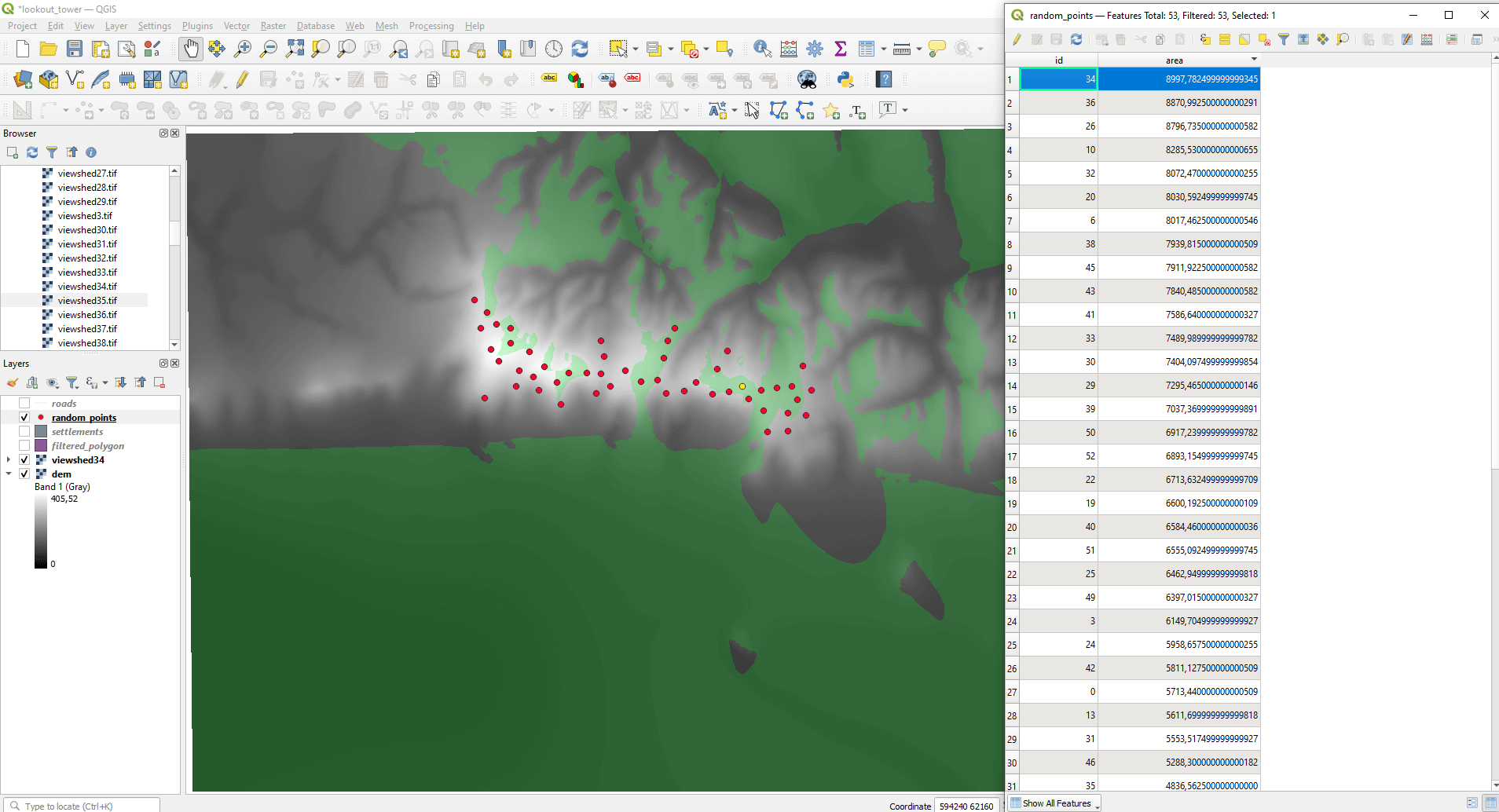
After you’ve run the code, the results can be easily read after opening the attribute table of the points. This can be done with choosing the “Open Attribute Table” option.

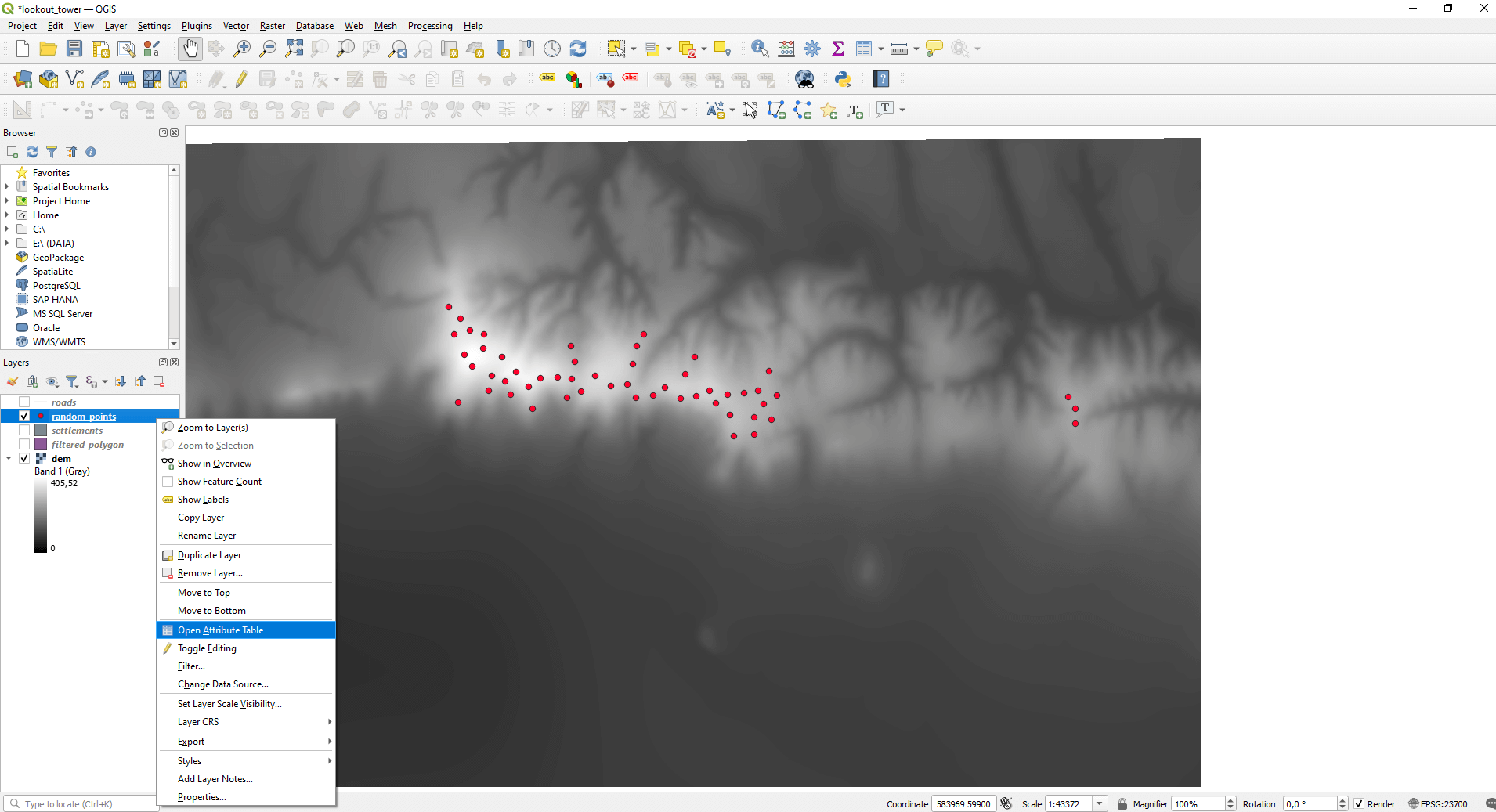
Double click on the header of the new “area” column to set the values in a descending order. So you only have to click on the number at the beginning of the line and then you can select the highest value. This means that this is the point with the highest viewshed. During the writing of the code, I defined the area units in hectares. 

CLOSING THOUGHTS

With this article, my intention was to promote process automation in an open-source environment. I hope this content will be useful to many. Feel free to use the codes presented here in any project. 🙂

If you really liked what you read, you can share it with your friends! 🙂

Did you like what you read? Do you want to read similar ones?