
There are many cases in different economic areas, when we face the challenge to calculate volume from point clouds or digital elevation models (DEM). One of the most common cases of this calculation is when we want to determine the volume of a material depot based on purely geometric data.
A large, accurate point cloud and a digital elevation model (DEM) are essential for volume calculation. These and the results of the calculation can be difficult to share with the client and colleagues. It is highly recommended to use the SurveyTransfer data sharing software! For more information, visit the software manufacturer’s website by clicking HERE.
A key question in the calculation is the resolution of our models, as the more accurate they are, the better results we can get. Furthermore, the way we perform the calculation is also an essential question. It is possible to measure the volume of material depots on a point cloud or a DEM based on a single survey with respect to a fictitious plane (assumed ground level). In addition, the differences between the models recorded at different times can also be calculated based on point clouds and DEMs. I have given examples for each of the four cases, which I will describe as a guide, so you can try them out.
To present the calculation I used open-source software which you can download and install. For analyzing point clouds I used CloudCompare, while for analyzing DEM files I used the 3.22.1 version of QGIS.
The purpose of this article is to explain the basics of soil mass calculation in such detail that what is described here can be applied in a simpler project. However, I would like to point out in advance that there are several complex cases, so don’t just blindly click through the session I’m presenting to you, but always consider whether or not you got realistic data back. As a test, it is worth taking a measurement with a regular geometry – one that you know the exact volume of – and testing the methods on this.
For the presented methods I used Mark Hamilton’s model which is available on Sketchfab. The model is under the license of Creative Commons, therefore, it can be used for free. For analysis, the model was also transformed into a point cloud and a raster.
1. EXAMINING A POINT CLOUD WITH A SIMPLE PLANE
In this chapter, we use CloudCompare to determine the volume of a depot based on a simple plane and data from a point cloud above the plane. In the point cloud, we first cut the material depot together with its surroundings and then break it down into further parts. We derive a plane from the environment of the material depot, from which the volume of the depot is calculated.
Sidenote: In CloudCompare, it is possible to automatically sort soil level, buildings or vegetation with a plugin called CSF Filter. This procedure is very useful if you want to create building models for cities or just create a terrain model. If you are interested, be sure to try the CSF Filter plugin, as it is a great way to automate workflows with it. Of course, it is also excellent for filtering depots, but I will show you a manual sequence of operations below. Manual settings are unavoidable in some cases, and so the presentation will not consist of at least just two clicks thankfully. 🙂
Open CloudCompare and import the point cloud (“Open”).
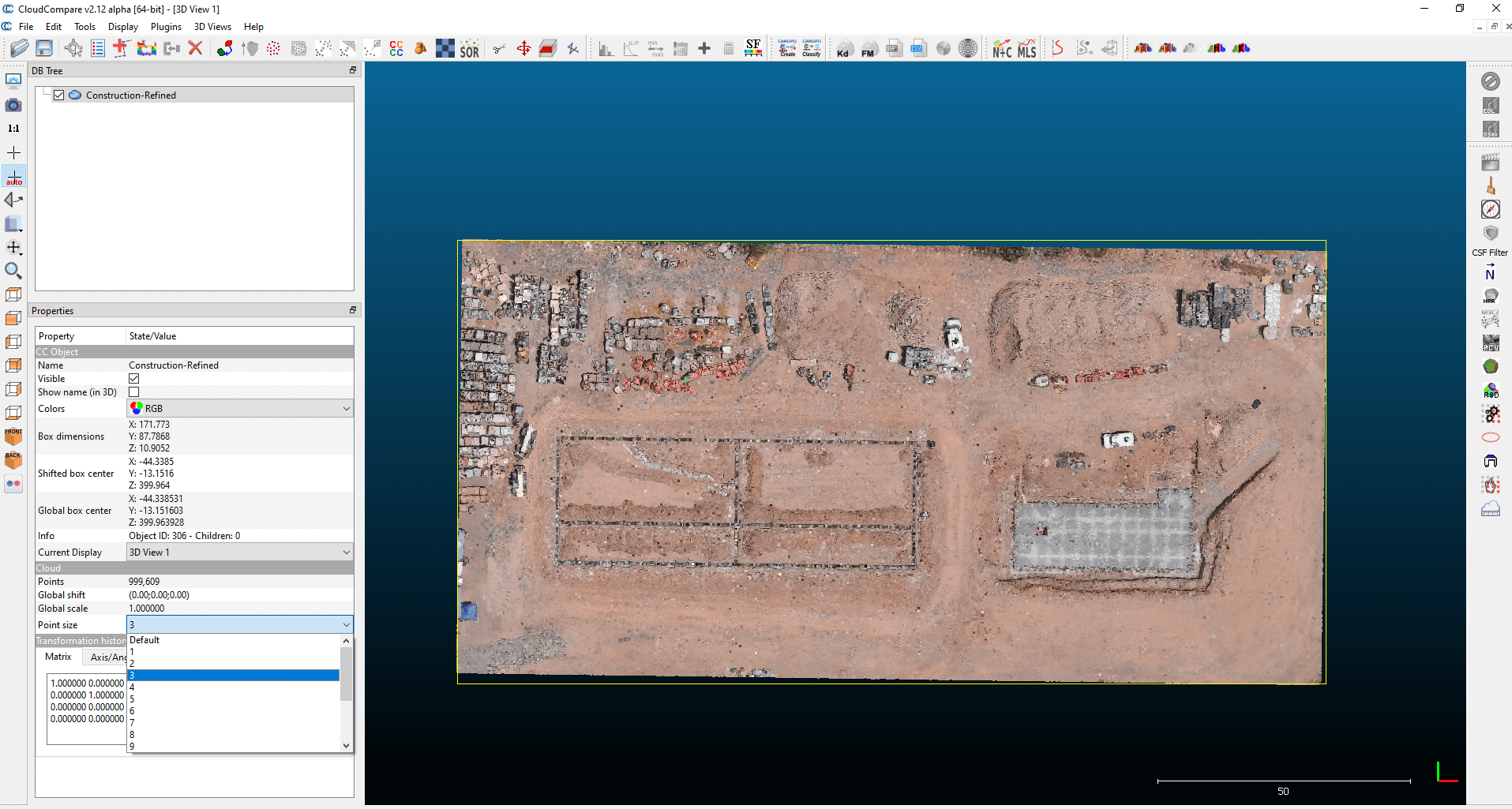
There are some adjustments we need to make before the calculation. First of all, increase the size of the points to make them more visible with higher zoom levels. Select the point cloud layer, then under the layer tree (“DB Tree”) the “Properties” window will appear in which you can find the “Point size” dropdown list. Optionally set a point size that is conveniently visible to you. 🙂
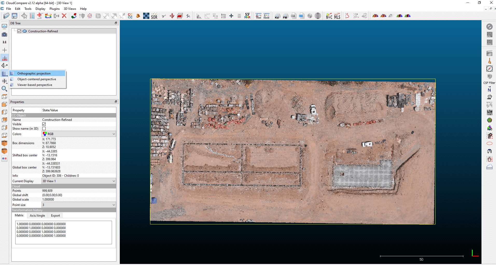
Now choose the “Set current view mode” menu from the left sidebar. In this menu, choose the “Ortographic projection” option. If you clicked, “Perspective OFF” will appear in the lower left corner of the model space. This is necessary because it prevents perspective distortion in the model and allows for a more precise delineation of the material depot. For easier navigation, press key “8” inside the model space, so you can view the model from above in a map view. In order not to accidentally rotate the camera while navigating, I advise you to move the camera by pressing the right mouse button. You can use the mouse wheel to zoom in and out on different parts of the model.
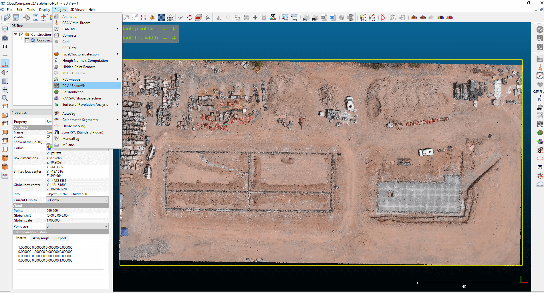
Finally, a few more display settings that can help delineate the material depot are the shadow effects. Select “PCV / ShadeVis” under the “Plugins” menu in the top menu bar.
Run at default settings unless the survey was carried out at the southern hemisphere (if it was, uncheck “Only northern hemisphere (+ Z)”). The result will be a grayscale model that reproduces the contour of the depots much better.

Also select the “Hough Normals Computation” add-on from the “Plugins” menu.
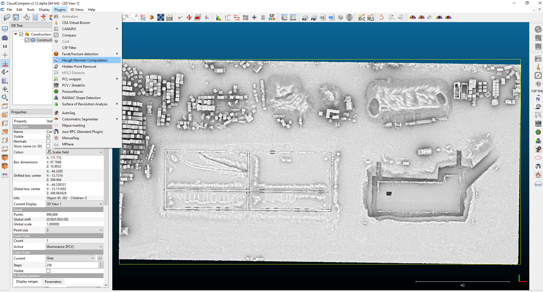
By running this on the default settings, the outline of the depots will be even more conspicuous, as it will calculate the normal, i.e., the orientation, of the points.
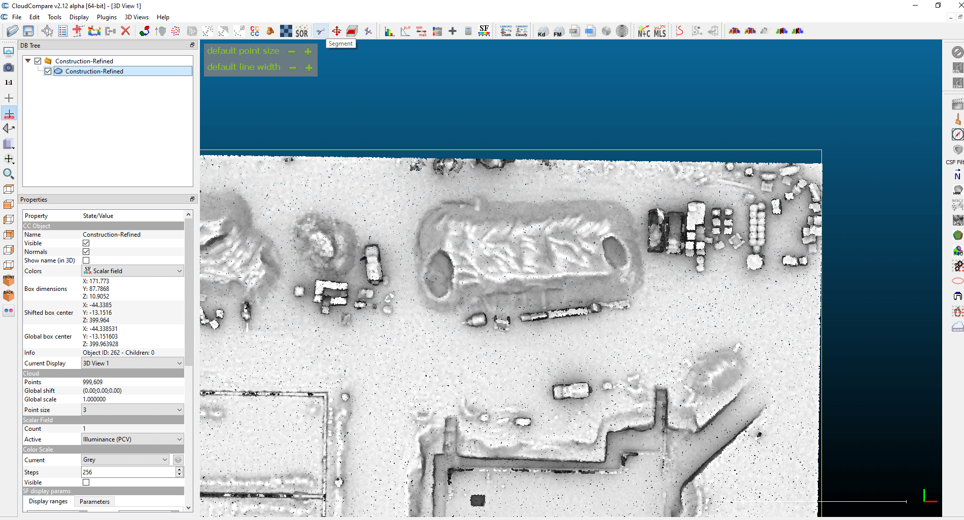
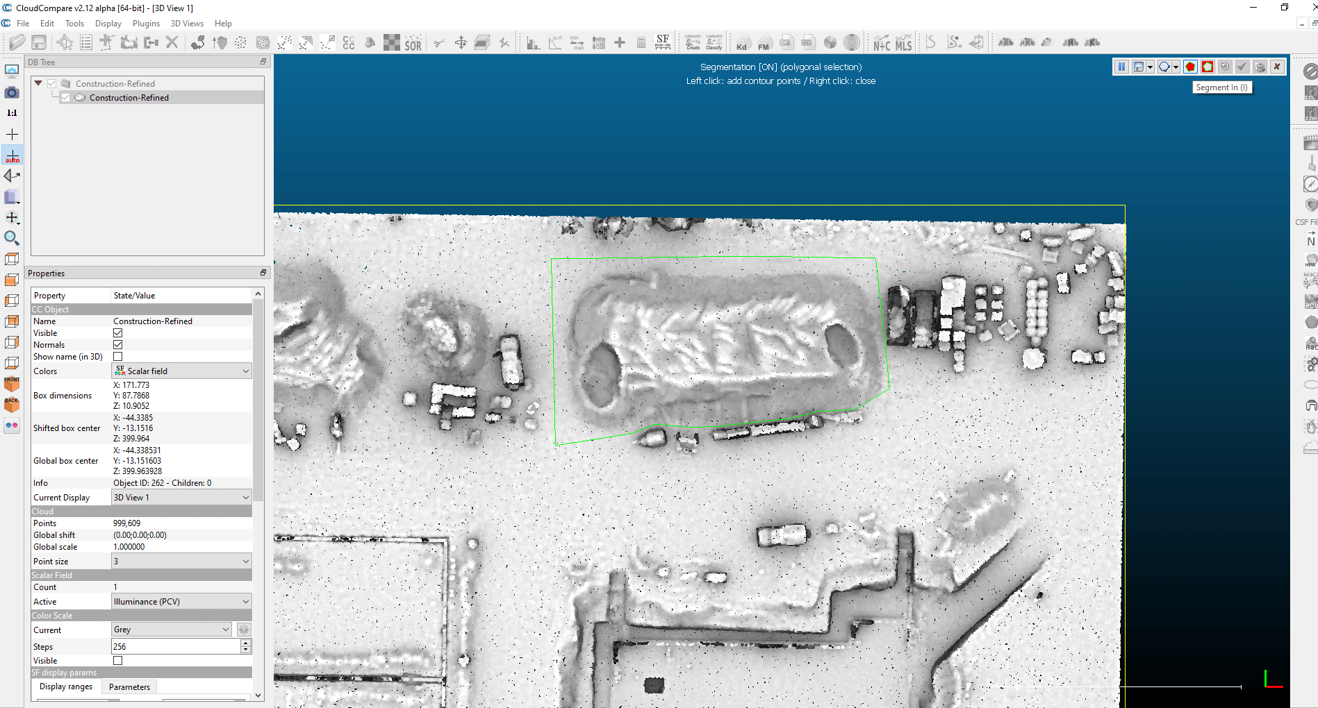
You can then start outlining the depot manually. Select the point cloud layer, then click the scissor icon (“Segment”) in the menu bar.
Left click to outline the depot around it, selecting points from the ground level as well. Do not rotate the camera in this part, as this outline can only be interpreted in 2D! An area with a green outline appears here. When you are done, press the right mouse button to finish editing.
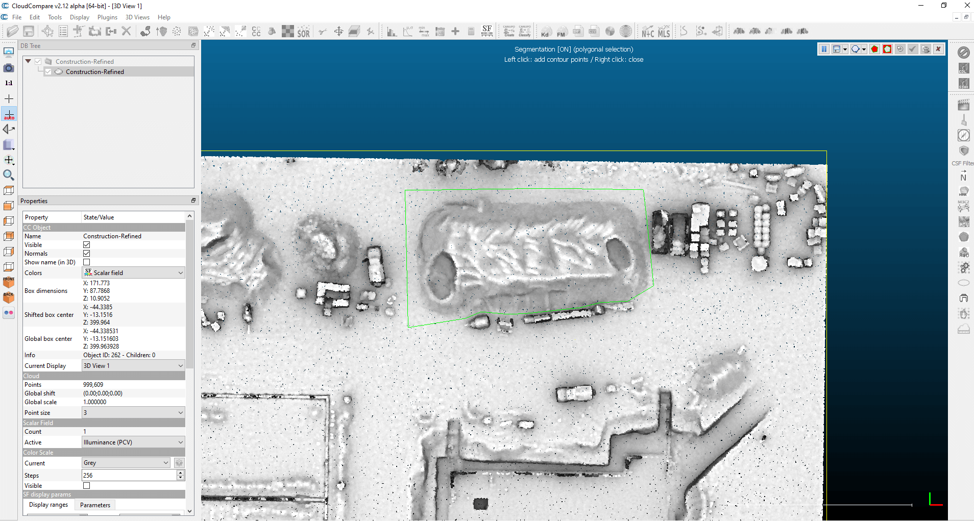
Select “Segment In (I)” from the drawing toolbar.
Then click the “Confirm segmentation (Enter)” button with the green check mark icon.
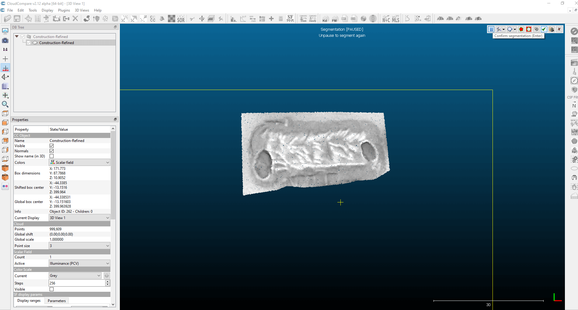
Two new layers have appeared, one with a name ending in “.remaining” and the other in “.segmented”. We’ll deal with “.segmented” below, so turn off the visibility of the other layer.
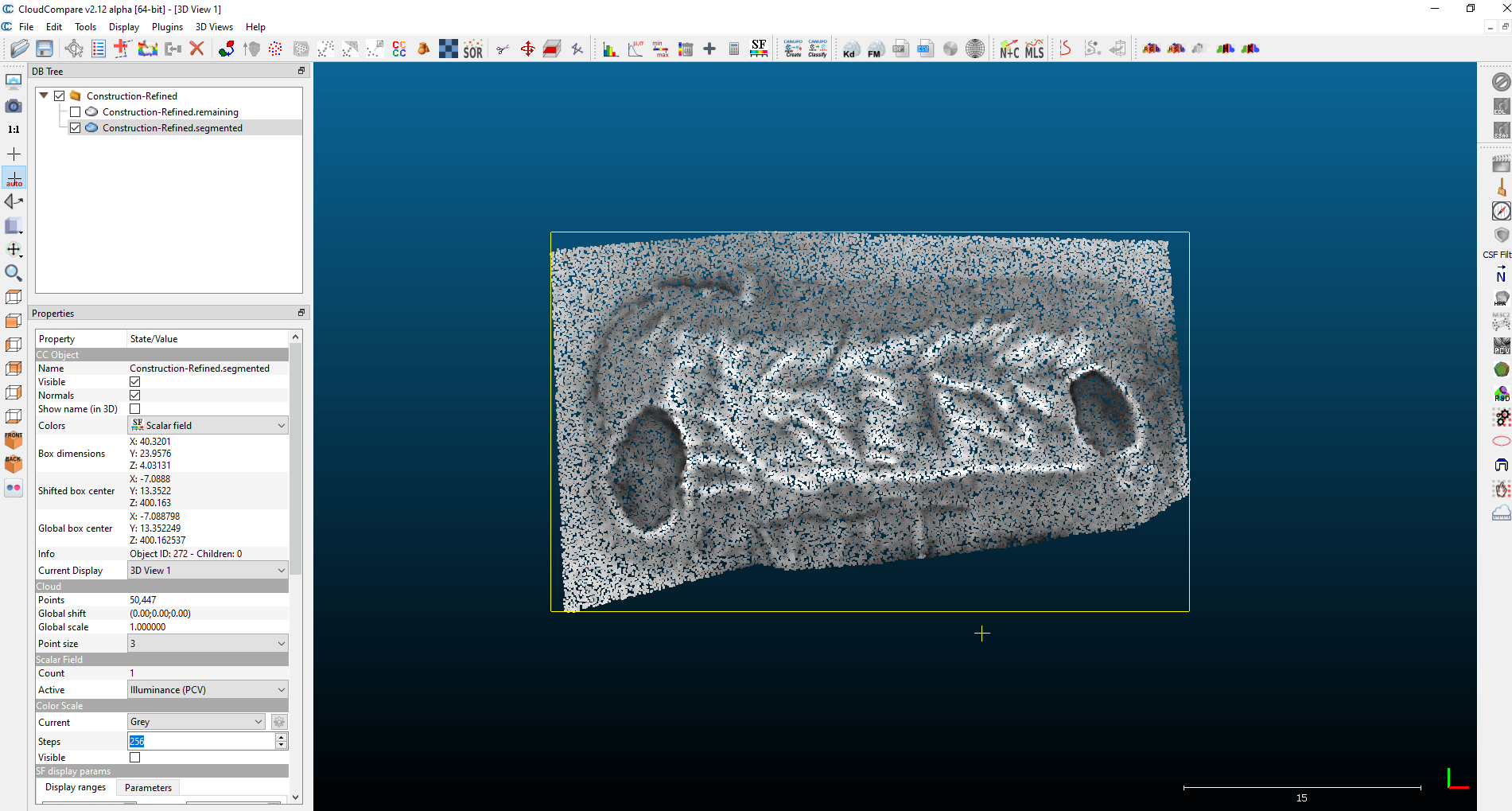
We also segment this layer. In this cut, you are already actually drawing the outline of the depot.
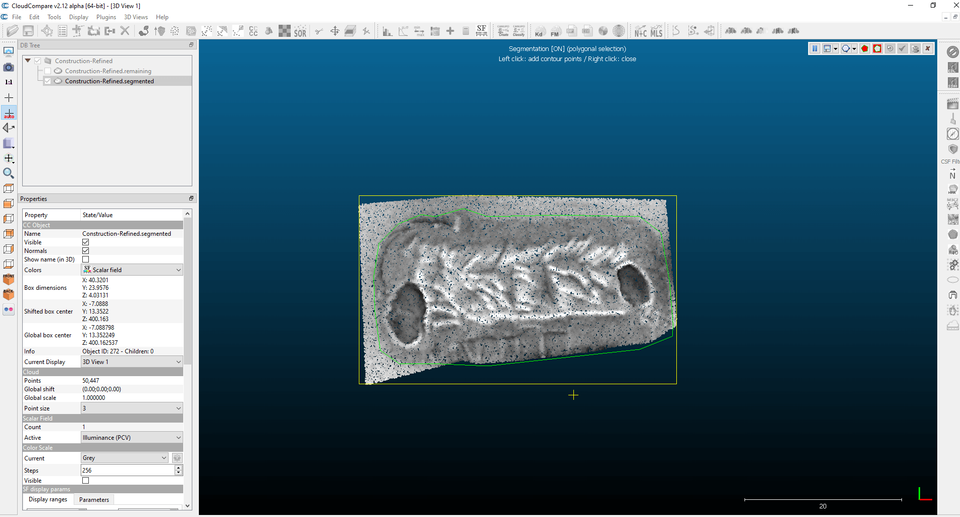
Now we’re going to add a plane to the layer, the name is a bit confusing, called “.segmented.remaining.” Select the layer, then select “Fit” from the “Tools” menu, and then the”2.5D quadric” option.
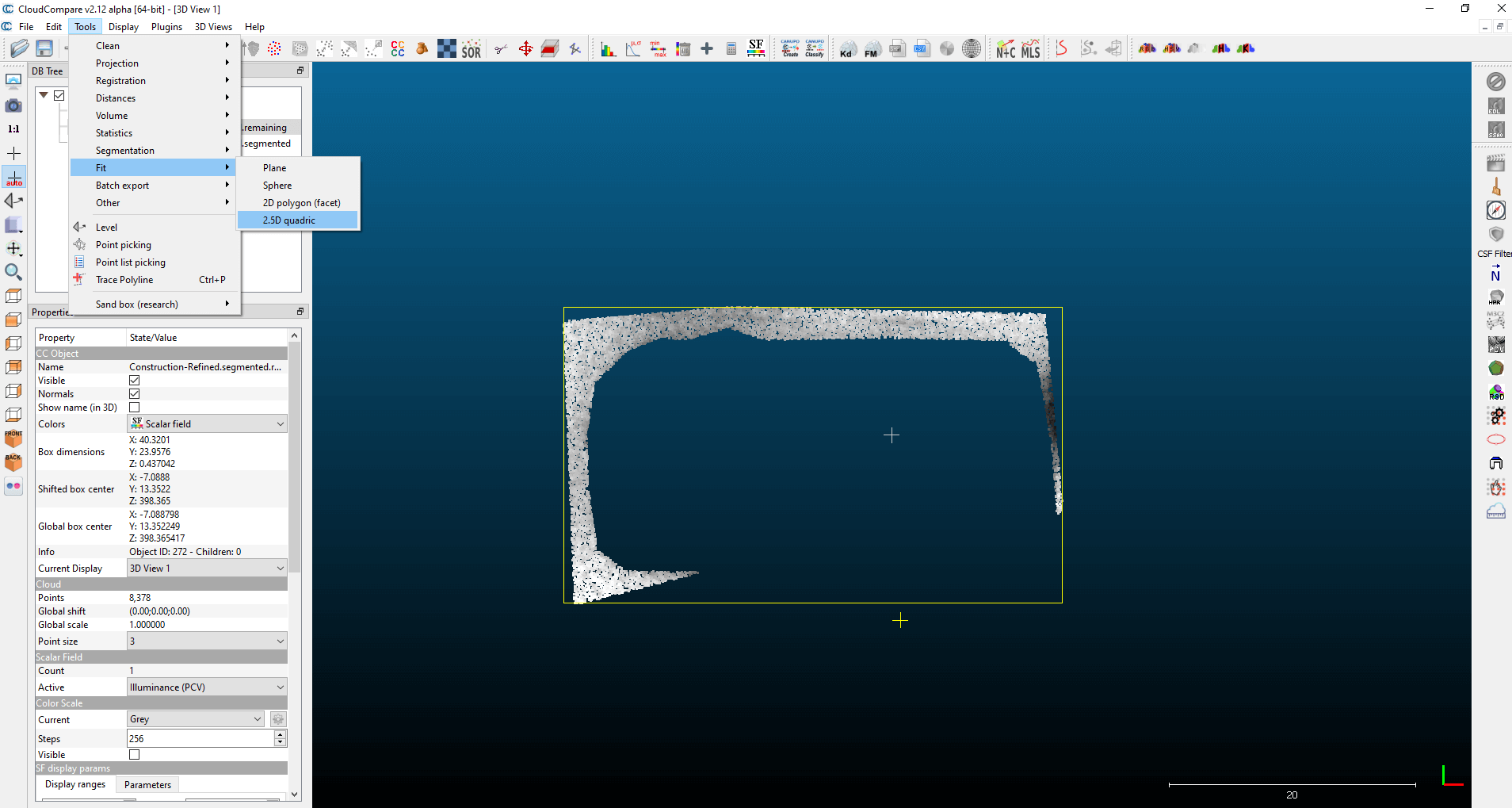
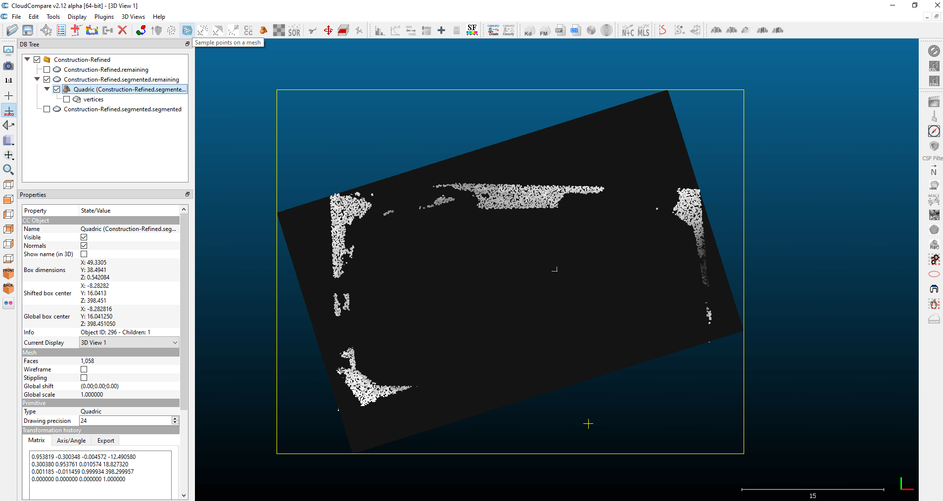
The superimposed plane appears immediately, but this is not a point cloud, and under CloudCompare we can only measure volume between two point clouds. Transform the plane into a point cloud. Select the “Quadric” layer, then click “Sample points on a mesh” in the top menu bar. You can run the function even with the default settings.
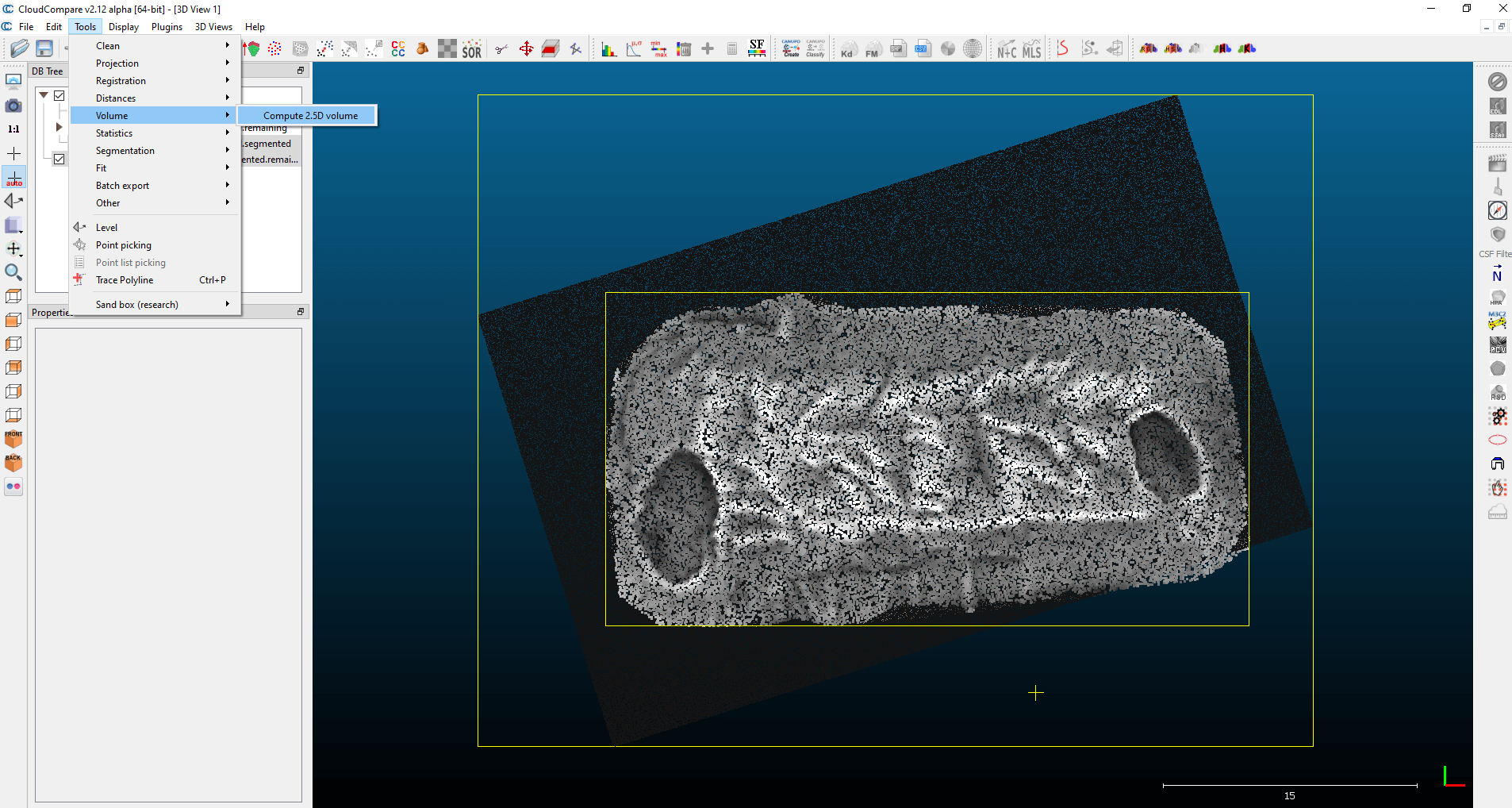
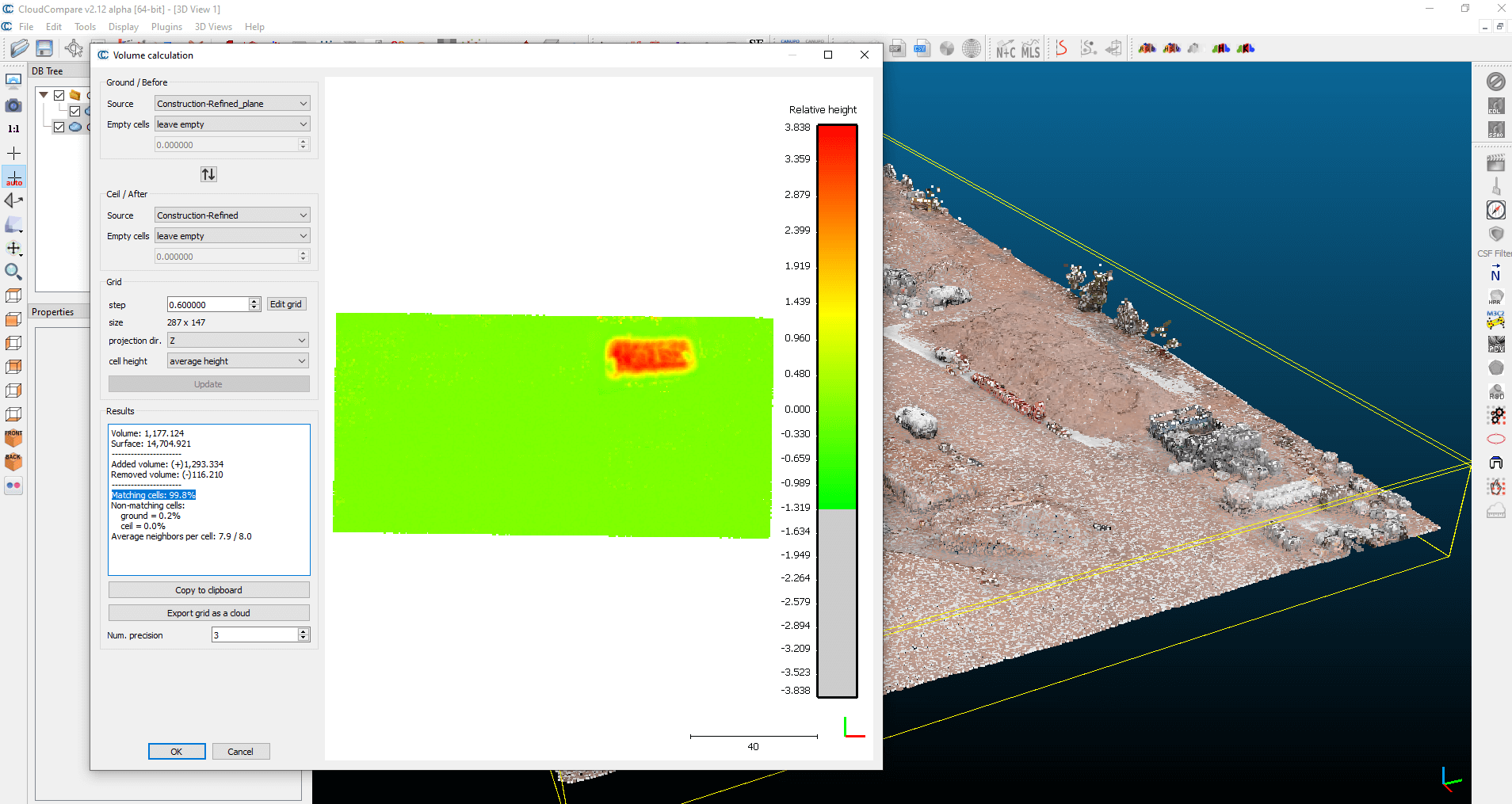
Select the newly created point cloud and the segmented material depot by pressing “Ctrl + left mouse button”. Under the “Tools” menu, select “Volume” and then “Compute 2.5D volume”.
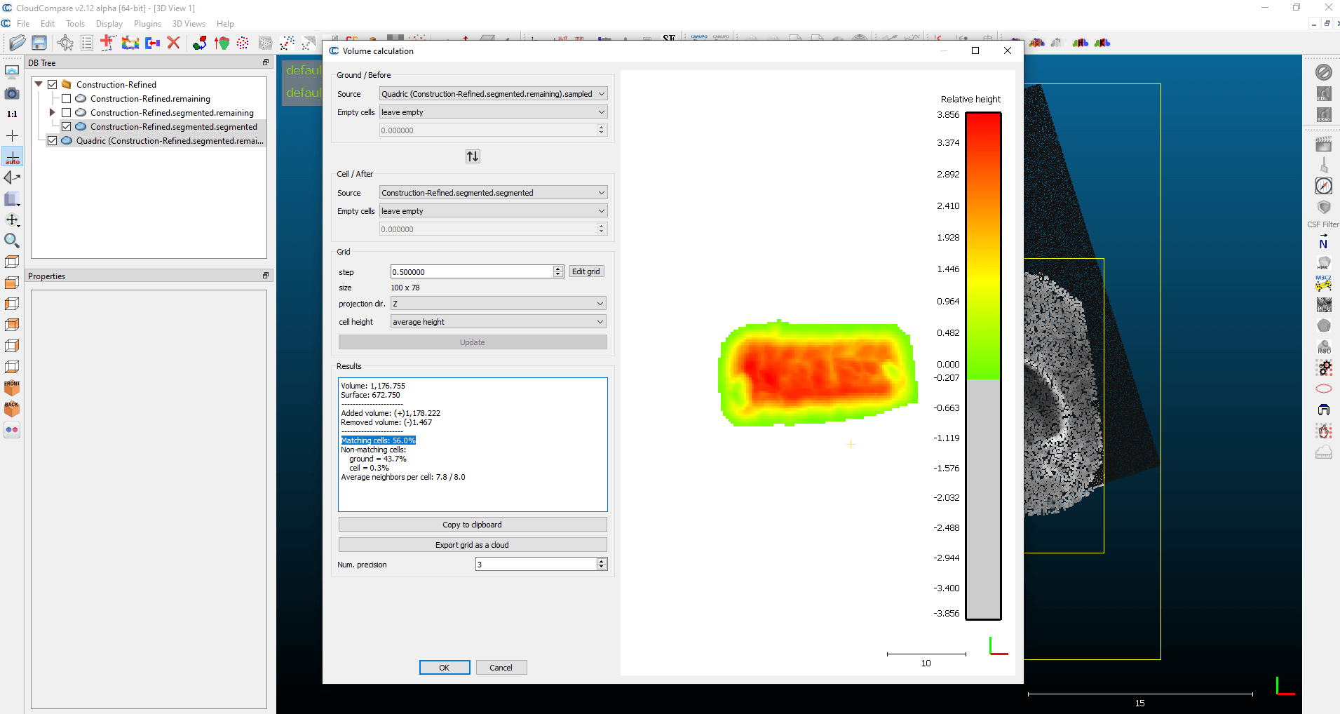
Under “Ground / Before” enter the “Quadric” point cloud layer and under “Ceil / After” enter the depot layer. In the “Grid” window, the value of “step” will be one of the most important variables! Experiment with this to see which value will work. How can you tell that? Good question! After clicking on the big red “Update” button after setting a value, the calculated surface, the added and extracted volume and one other important data called “Matching cells” will be displayed in the “Results” window. Try increasing or decreasing the “step” value until you get the highest “Matching cells” ratio. The more raster that fits in space, the more accurate the calculation will be. Yes, this function results in a raster calculation.
2. CALCULATING VOLUME BETWEEN POINT CLOUDS
I present the second calculation method between two point clouds, also in CloudCompare. This one is much easier to perform, I will show you why.
Sidenote: Even though this calculation method is faster and simpler, you really need to pay attention through data collection that the Ground Sample Distance (GSD) needs to be almost the same in case for both point clouds. In addition, the spatial position must be taken into account, so great emphasis must be placed on accurate georeferencing!
Open both point clouds in CloudCompare, select them and then start the previously presented “2.5D Compare” function. In the “Ground / Before” section, set the point cloud where there is no material depot yet, while in the “Ceil / After” section, select the layer with the depot. We can achieve a much higher “Matching cells” value if the data collection and georeferencing were good.
If you have looked closely at the result at the end of the previous chapter, you can see that there is a difference of 115,112 m3 between the volumes added. This is because we have made the calculations for the whole point cloud. In this case, too, it is possible to segment the point clouds, i.e., to cut only the material depot to be examined. Now it can be seen that the difference is only 8.897 m3 so, the difference between the two calculations significantly reduced. Even though the two calculations are quite close to each other, the calculation between point clouds can be considered more accurate, as the value of “Matching cells” is much higher. Thanks to the two-phase data collection, we have more data on the soil level, i.e., the state without a depot.
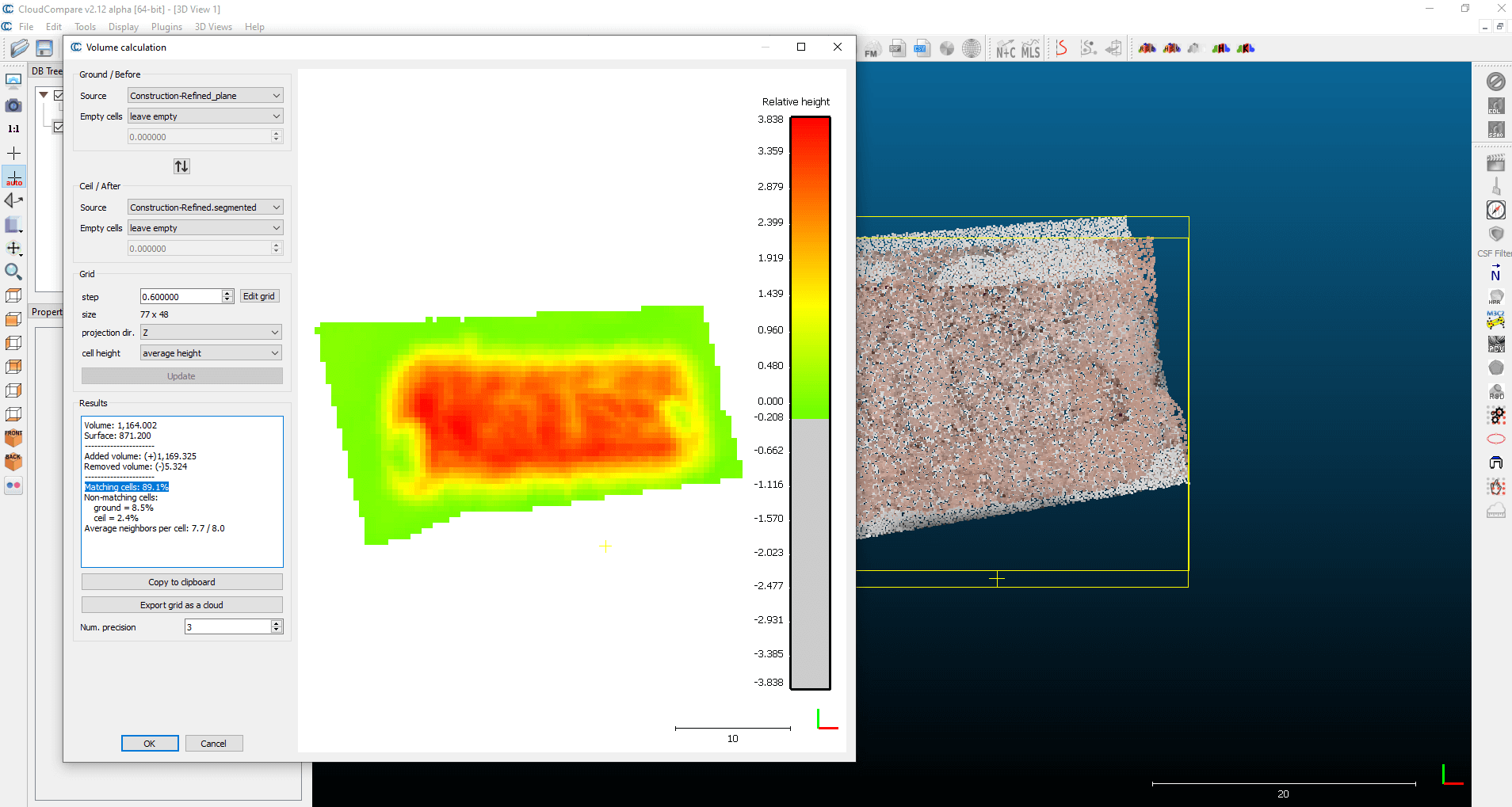
Sidenote: In the “Compute 2.5D volume” function, “Empty cells” can also be set for both files (“Ground / Before” and “Ceil / After”). This applies to empty cells that cannot be read from the point cloud. Here it is worth trying the “interpolate” option, which uses a geostatistical calculation to determine the expected values of the intermediate, data-missing parts. This means that even if data is missing, the software estimates the expected values. With this setting, we can get even higher “Matching cells” ratios and thus I got an even closer value to the calculation done in the previous chapter.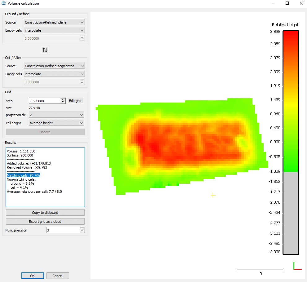
3. DEM VOLUME CALCULATION ALONG A PLANE
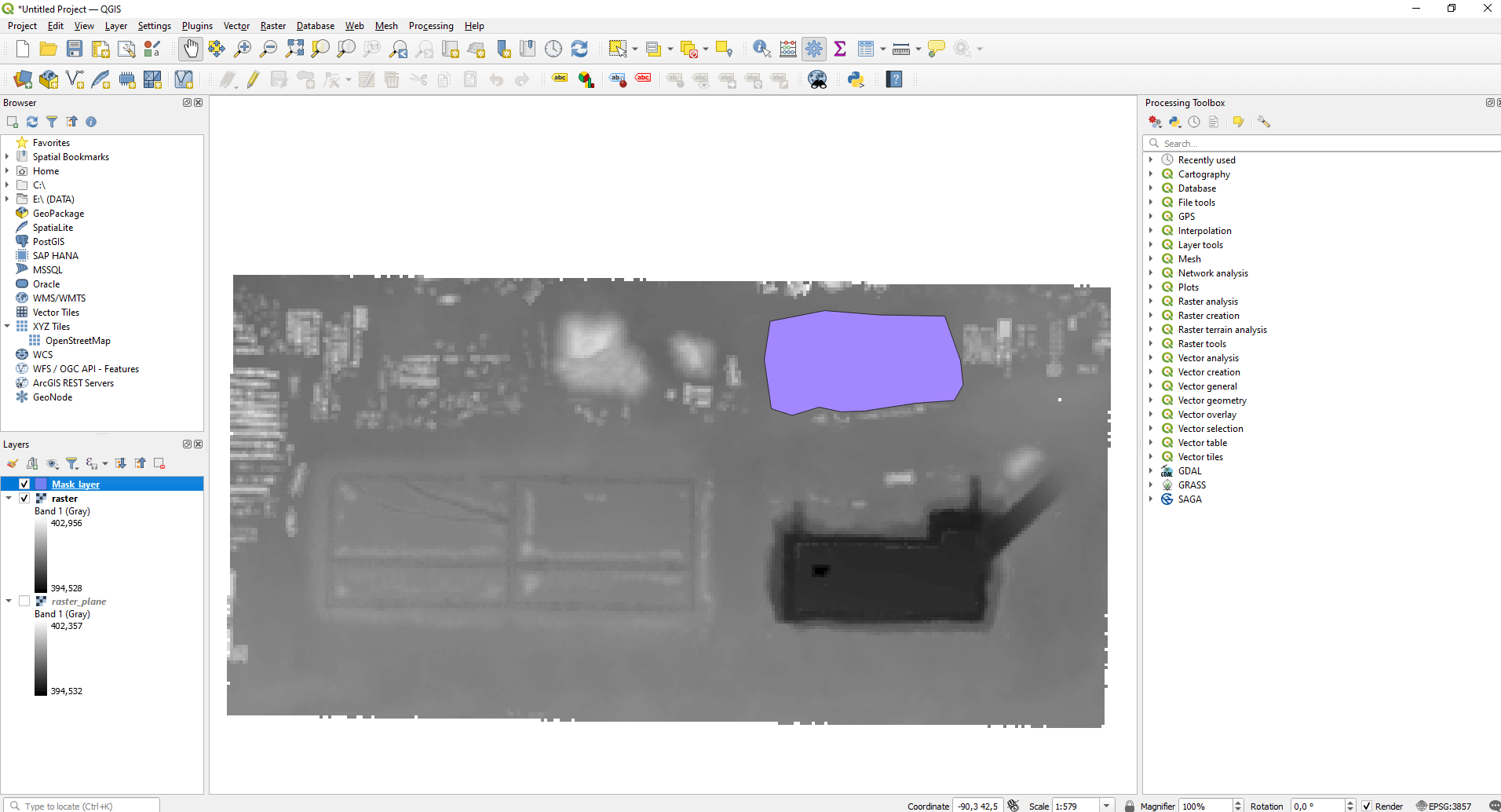
Now we will leave the magi wrold of CloudCompare and open QGIS. We are going to analyze the presented model. The only difference is that we now analyze it as a raster file. If you have only one DEM and you want to calculate a volume from it, you have to specify a plane, relative to which the volume of the object can be calculated for the parts below or above it. Open QGIS, then locate your DEM file in the “Browser” window on the left and add it to the map using drag-and-drop.
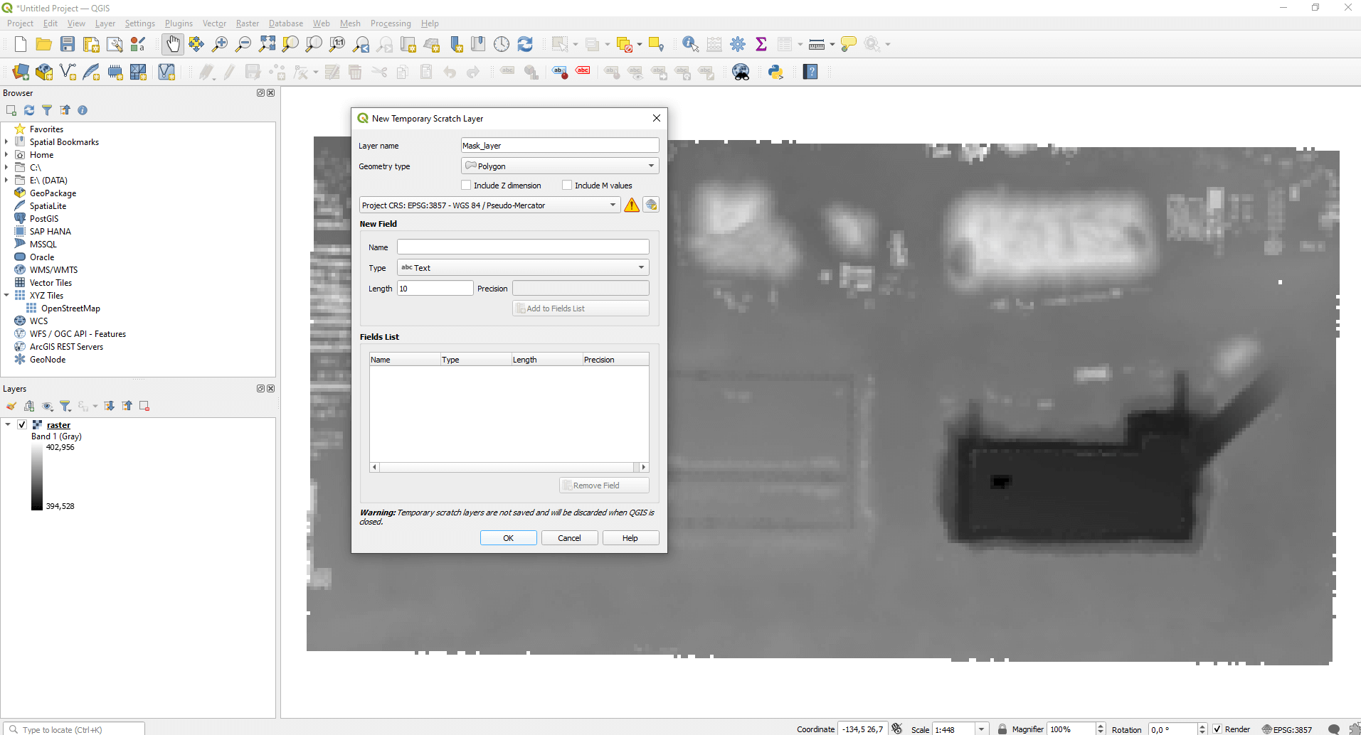
As the starting step of the calculation, we need to determine the offset of the plane that sets the starting level of the calculation. The volume of the space above this level will be calculated. The simplest way is to trim the material depot in this example as well. Create a new polygon layer with which we can cut out the depot! Select “New Temporary Scratch Layer” from the top menu bar.

Enter a name for the new layer, then select the “Polygon” geometry type, set the coordinate system in which the DEM was created, and finally click “OK”.
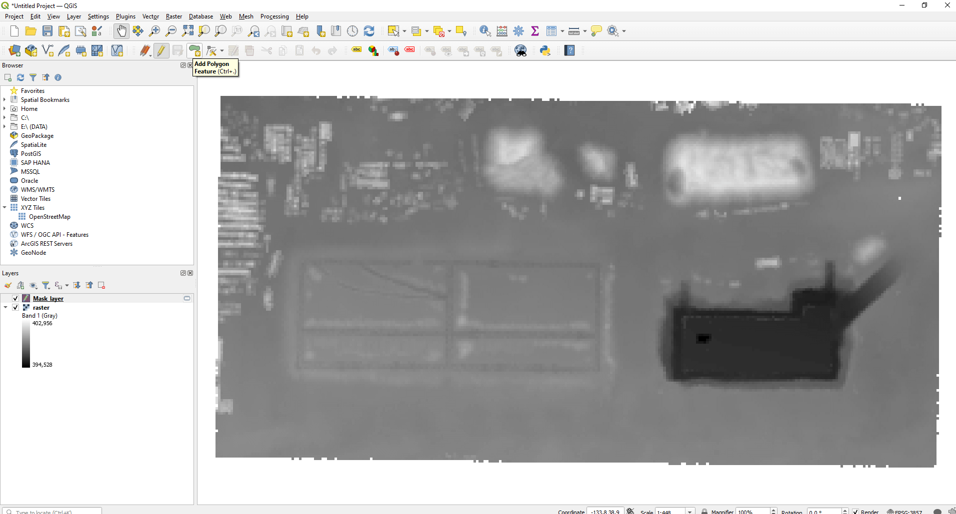
Editing mode automatically starts on the new layer, so you can start drawing the area by clicking the “Add Polygon Feature” button in the top menu bar.
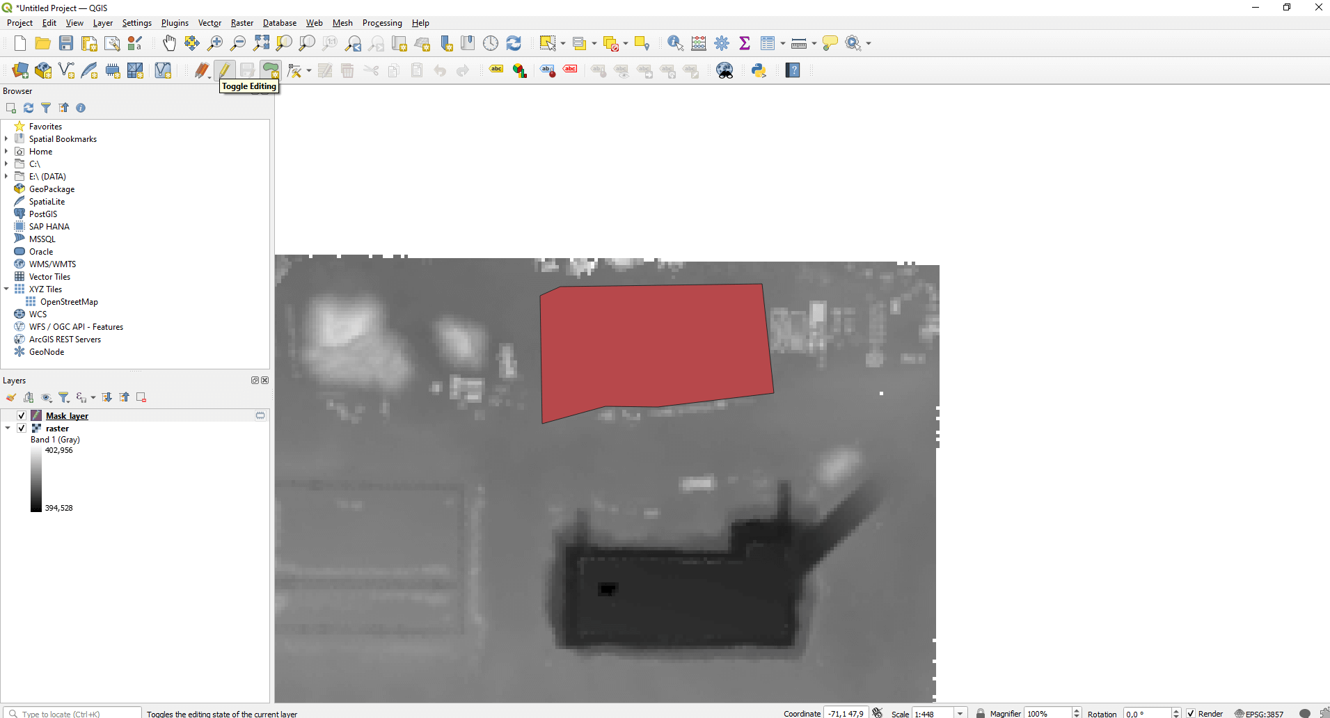
You can left-click to place polygon breakpoints, and then right-click to close the area. Then save the layer with the “Save Layer Edits” button.

Finally, complete the editing process by clicking on the pencil-shaped “Toggle Editing” icon.
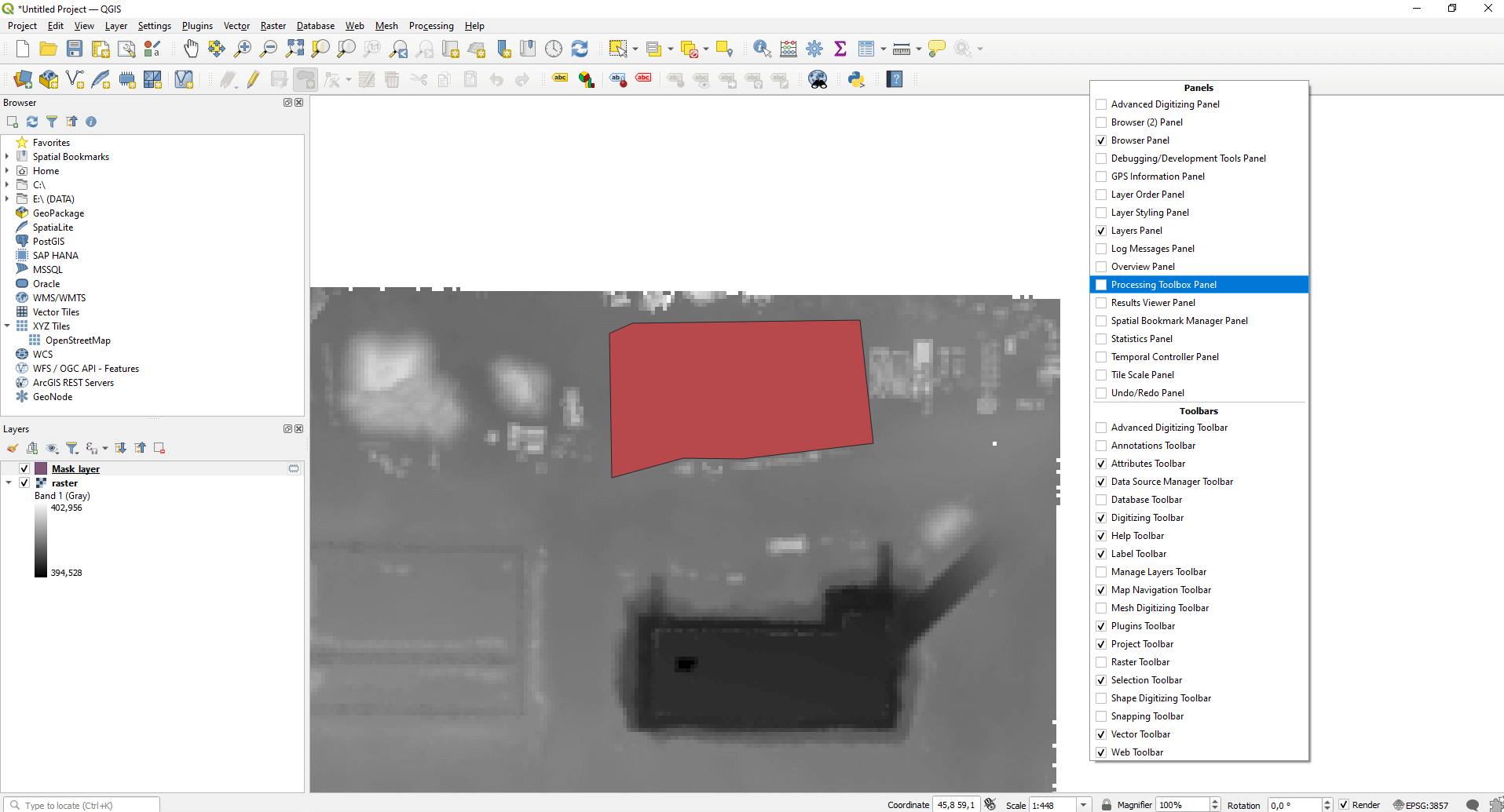
Right-click on the menu bar and activate the “Processing Toolbox Panel” window.
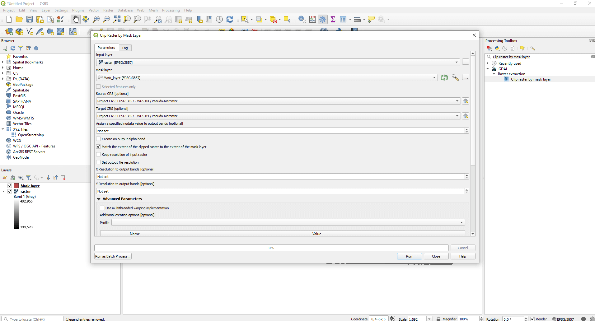
Search for “Clip raster by mask layer” in the search bar and choose the first GDAL function. In the window that appears, enter your raster file and then the area from which you want to cut the DEM. When you are done, press the “Run” button. In a nutshell, the function works by converting the vector area into raster cells and then saving the mutual points of the overlapping rasters to a new layer.
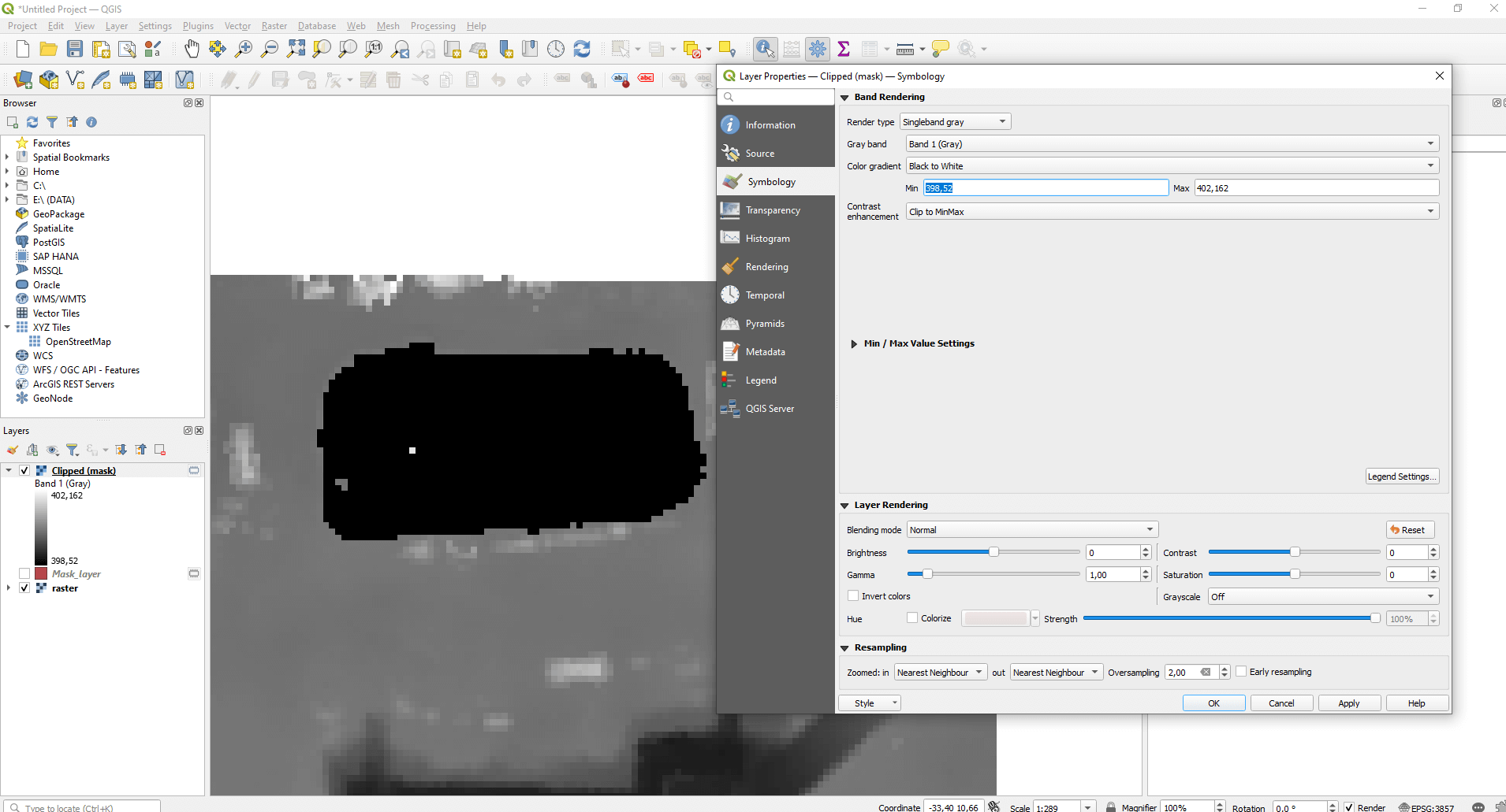
The lowest point of the appearing raster file can be read from the layer tree. In this case it is 398.163986 meters, however, I recommend not to use this value when defining the plane, because it can be misleading. Double-click the cut raster layer and the “Layer Properties” window will appear. Within this, select the “Symbology” tab on the left, then select “Clip to MinMax” from the “Contrast enhancement” drop-down menu. After all this, start increasing the value “Min”, then press the “Apply” button. Observe on the map at which “Min” value the black space covers most of the object. If it is completely obscured and there are no unnecessarily protruding areas, you have determined the height of the plane. For me, this value came out at 398.52 meters.
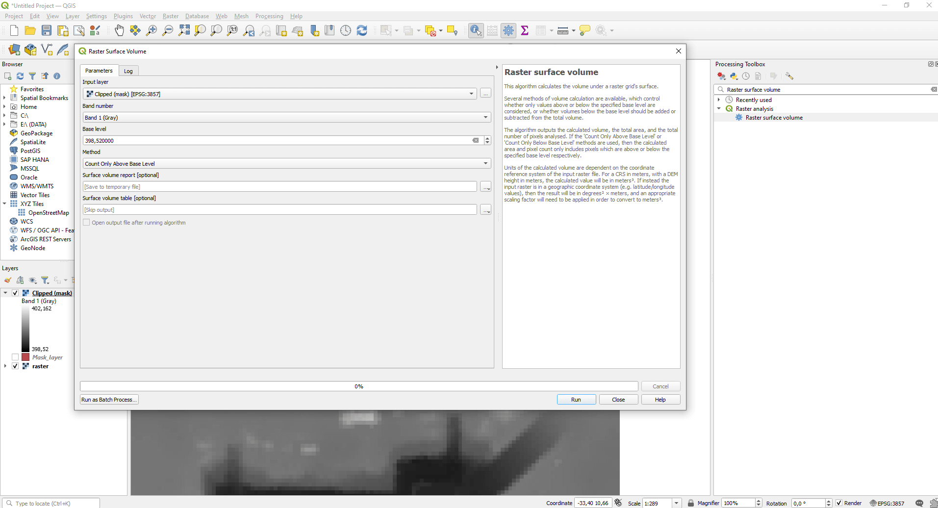
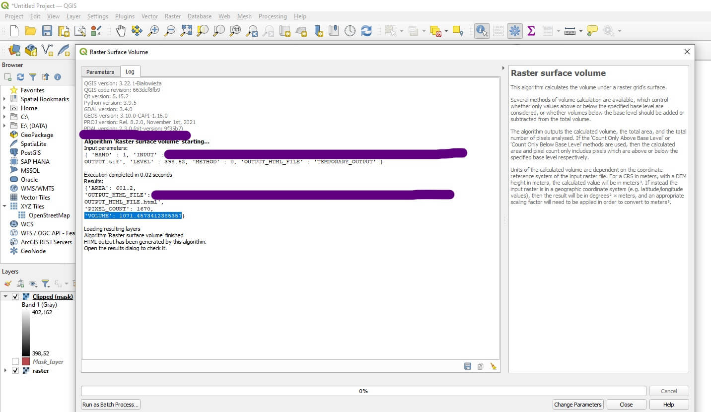
Search for “Raster surface volume” in the function search bar and double click on the first result. In the “Input layer” field, the previously cropped raster file must be entered, and in the “Base level”, the offset of the defined plane must be entered. Under “Method” you can choose from several options, for example, select “Count Only Above Base Level”.
The final result will be a report, containing the volume calculation. It is thought-provoking why the result was 106,765 m3 less than in the CloudCompare example, when we determined the mass of the soil above one plane in the same way. Well, there could be several reasons for this:
- CloudCompare uses a different rasterization algorithm, so DEM elevation data may differ.
- In the CloudCompare environment, we did not work completely flat, but with “Quadric” 2.5D geometry, so it had not just one-component elevation data.
- The resolution of the raster file may differ from the values derived from the point cloud.
4. COMPARING DIGITAL ELEVATION MODELS
In QGIS it’s possible to examine the differences between two rasters. Open the two files. Staying with the example, I will open DEMs, one of which is the result of a previous survey, that is, no material depot is yet visible on it, and one on which I already have the depot. Here we have to outline a circle around the area to be examined, as I have already shown in the previous chapter. I will not describe this in detail again, I will only show the result.
The easiest way to calculate volume between rasters is to install the „Volume Calculation Tool” plugin. You can install it by first clicking “Plugins” in the top bar and then “Manage and Install Plugins”.
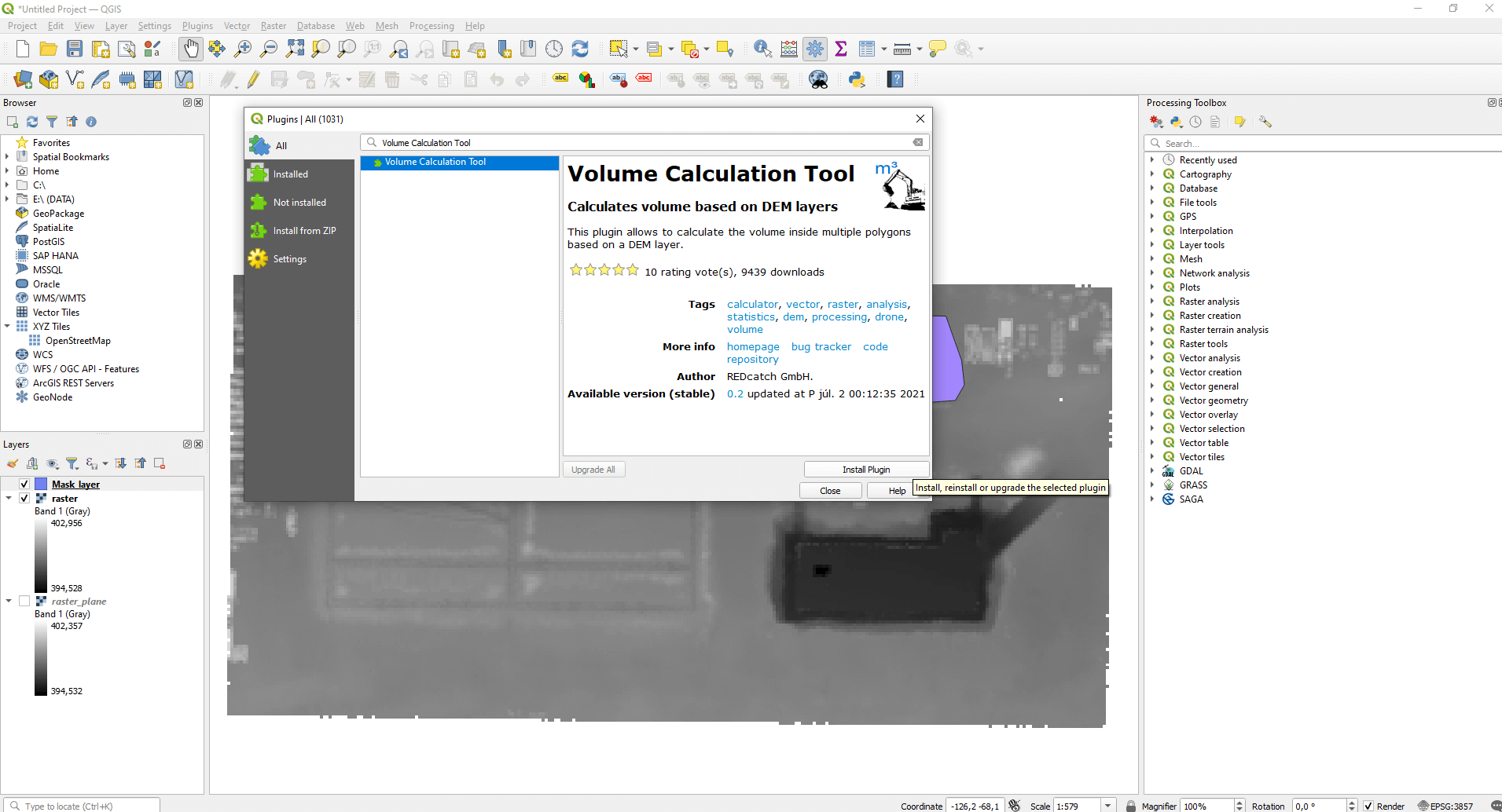
In the search bar type “Volume Calculation Tool”, then choose the plugin from the search results, then press the “Install Plugin” button in the bottom left corner. It will take a few seconds for the module to be successfully installed, then you can close the “Plugins” window.
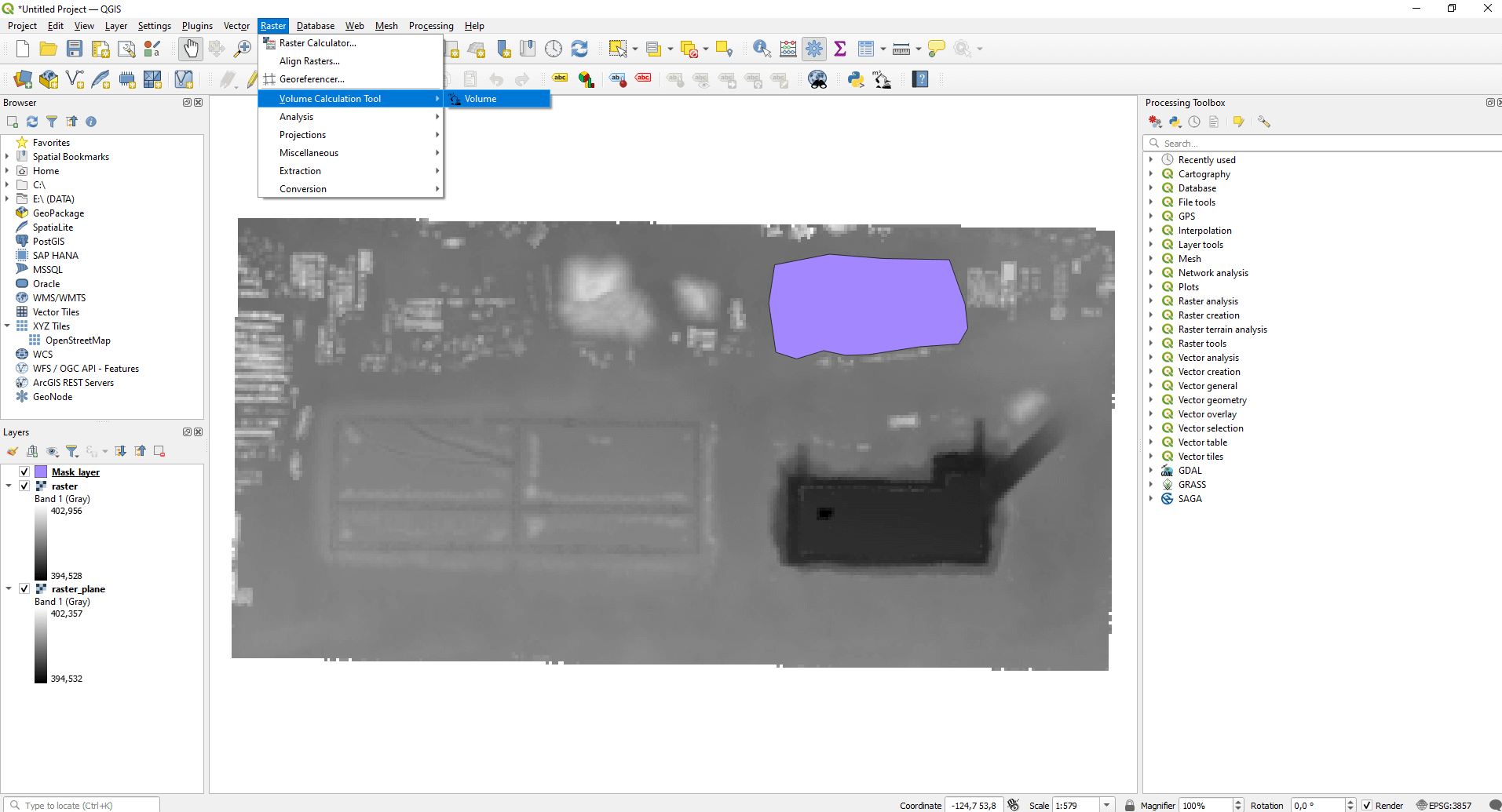
The new function (“Volume”) can be found in the top menu bar in the “Volume Calculation Tool” submenu, which is in the “Raster” menu.
In this tool, you must first specify the input layers, that is, the vector layer of the outline of the object to be examined (“Areas (Polygon Layer)”), and then the raster on which the material depot (“DEM Height Layer”) is visible. Within the “Define base level height” area, select “Use a SECOND DEM layer as a base” under “Choose type of base height”. Then enter the resulting raster of the previous survey in the “DEM Base Layer” menu item, where there is no material depot yet. Finally, under “Type of Volume Calculation”, set “Count only above (e.g., stockpile)” for “Counting Method”. Press the “Run” button. The result is displayed on the right.
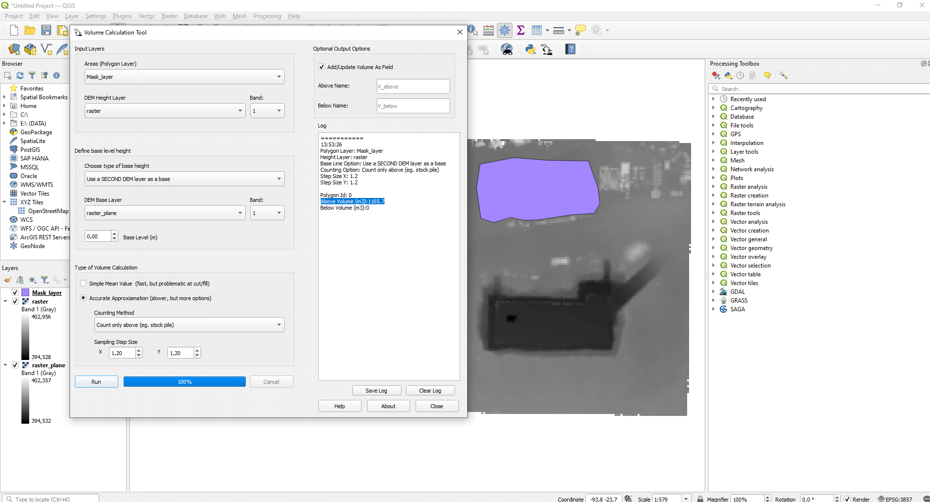
Sidenote: The “Volume Calculation Tool” would have been capable of performing the volume calculation along a plane, which was presented in the 3rd chapter. However, I wanted to show an alternative solution as well. This extension carries many opportunities, of which I have presented only one. With this, you can measure the volume of several material depots at the same time, thus making the calculation semi-automatic, as well as measuring an area with Z coordinates. If you’re interested in more about the other setup options and how they work, visit the developers ’website, or watch this YouTube video.
Summary
I thought it would be useful to summarize all the results of the different volume calculations so you can see how different the results of each method can be.
| Geometries used for calculation | Point cloud & Plane | Point cloud & Point cloud | Point cloud & Point cloud (interpolated) | DEM & Plane | DEM & DEM |
| Calculated Volume (m3) | 1178 | 1169 | 1171 | 1071 | 1166 |
This also shows that for a volume calculation to be effective, it is not enough to find a method that you just click through! It is necessary to know the possibilities and test, based on several sample areas, which method will be the most useful and accurate for a given project. I still advise you to select an object for which you know the spatial dimension and perform volume calculations on it. For example, make a 1m3 cube out of a cardboard box, measure it, and then try the methods described here.
If you really liked what you read, you can share it with your friends. 🙂
Did you like what you read? Do you want to read similar ones?