
In this article I will show you how to easily analyze a change of condition between two 3D objects. An example will present the motion of a building, meanwhile I will highlight the different opportunities and error factors.
I have done every step using open-source software, so feel free to try out all the presented methods.
To go through all the steps, you will need the following. For data preparation I used the Blender 2.93 version, and the BlenderGIS plugin. For creating data tables I chose the 3.22.1 version of QGIS. For the distance analysis of geospatial data, I used CloudCompare. The presented building model was made by Tomasz Armata. The model is free to use and available under the following link.
The goal of the article is to help your work. The knowledge presented on the following pages allows you to work on projects which require more complicated analyzes.
I recommend this article for those wanting to dig deeper into geoinformatics (and GIS). However, it can be useful for beginners who want to know what data analysis related challenges they might have to face through a project.
We won’t deal with data collection here. I assume that precise, and properly georeferenced data are available. Data which we only need to process and analyze.
What kind of files are needed for an analysis like this?
- We have two 3D models. One shows the initial condition, while the other shows the end state.
- Geospatial data can be analyzed as mesh and as point-cloud too
- The nature of geospatial data (point-cloud or 3D mesh model) can be used mixed. For example, the initial state can be a mesh model, while the recent state can be a point-cloud.
What are the steps through the process?
- Data preparation (if needed)
- 3D distance measuring between the two models
- Calculating bearing and tilt angles
- Visualizing data
CONSIDERATIONS BEFORE THE ANALYSIS
Before we get started, I must mention that this will mean two 3D distance-based measurements. And because of that we need to think of the correct steps to achieve the best results possible.
If you are about to compare two different object that:
- Have significantly different spatial locations. This means that, along several axes, one object is tilted and moved relative to the other. In this case we need to place reference points on the models and analyze the distances between them.
- Almost have the same location but some parts are missing from one of the models, we can analyze the deviation along the surfaces.
There is only one big difference between the two. While in the first case you will get as much data as the number of the reference points, the second case will result in a mass data set. It is worthy to make statistical reports about this mass data set.
In the first case it’s best to use Blender for creating reference points. In the second one you won’t need Blender.
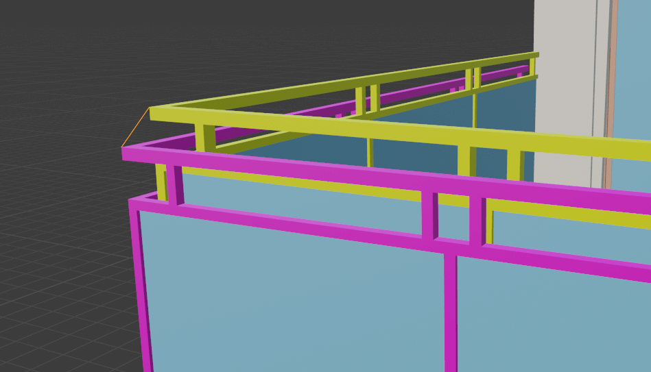
You still don’t understand why you need reference points in some cases? Let me explain this through an example. The following image ummarizes the essence of it.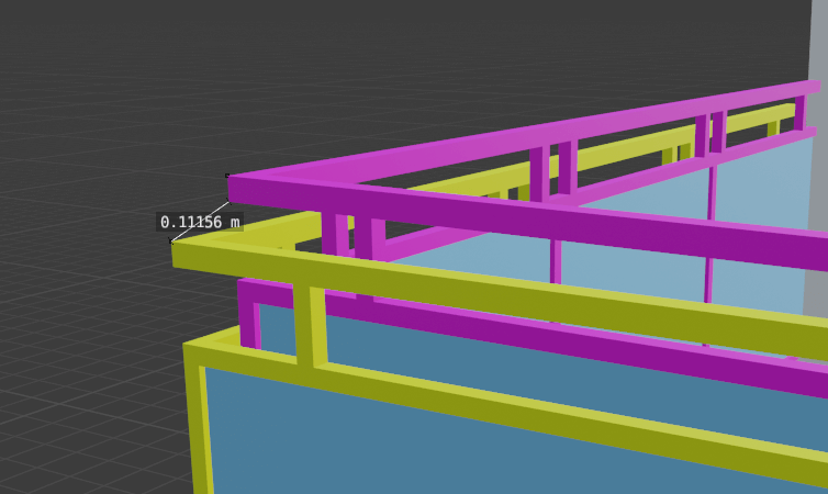
We want to compare the building with the yellow railing to the other one with pink railing. We can clearly see that they differ in space so much that the bottom of the railing on one model is closer to the top of the railing on the other one. It’s evident that in both models we want to compare either only the points belonging to the upper level, or only the points belonging to the lower level. If the comparable points are mixed up, the algorithm that calculates the shortest distance will show a wrong result. And it may cause great confusion if you calculate the direction and the inclination of the tilt of the object based on incorrect data.
PLACING REFERENCE POINTS
In this chapter we analyze the first case when it is inevitable to place reference points in the model and use them for distance calculation.
SETTING UP BLENDER
Of course, the first step is to install Blender. It’s quite simple so we won’t discuss it in depth: Next, Next, Finish… Install BlenderGIS! In this site, under the “Code” button you take the “Download ZIP” option.
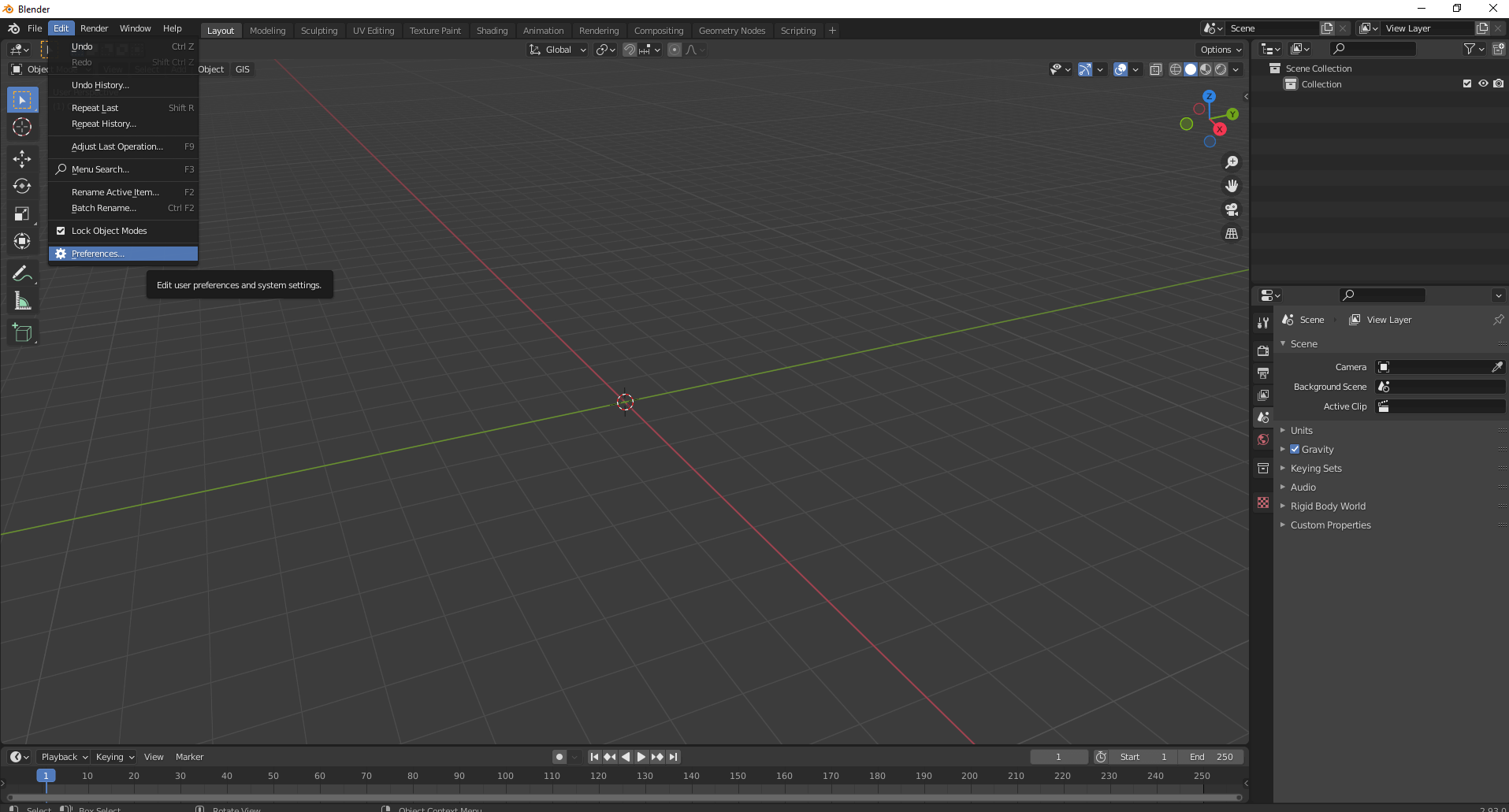
Now open Blender. Click next to the welcome window to make it disappear. We will work in an empty model space, so select every object with the “A” key and delete them with the “Delete” key. If the BlenderGIS plugin isn’t installed yet, you can install it under “Edit/Preferences” in the top menu bar.
Choose the “Add-ons” option from the left sidebar, then choose the “Install…” button from the upper part of the menu. Here you pick the “.zip” file you have just downloaded. If the installation was successful, the plugin will appear.
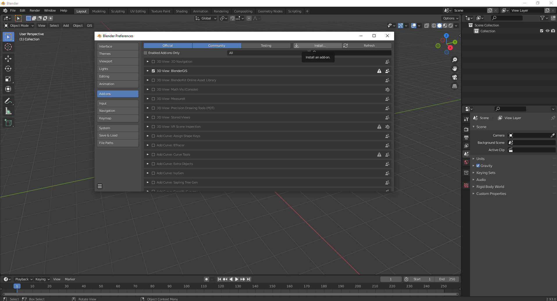
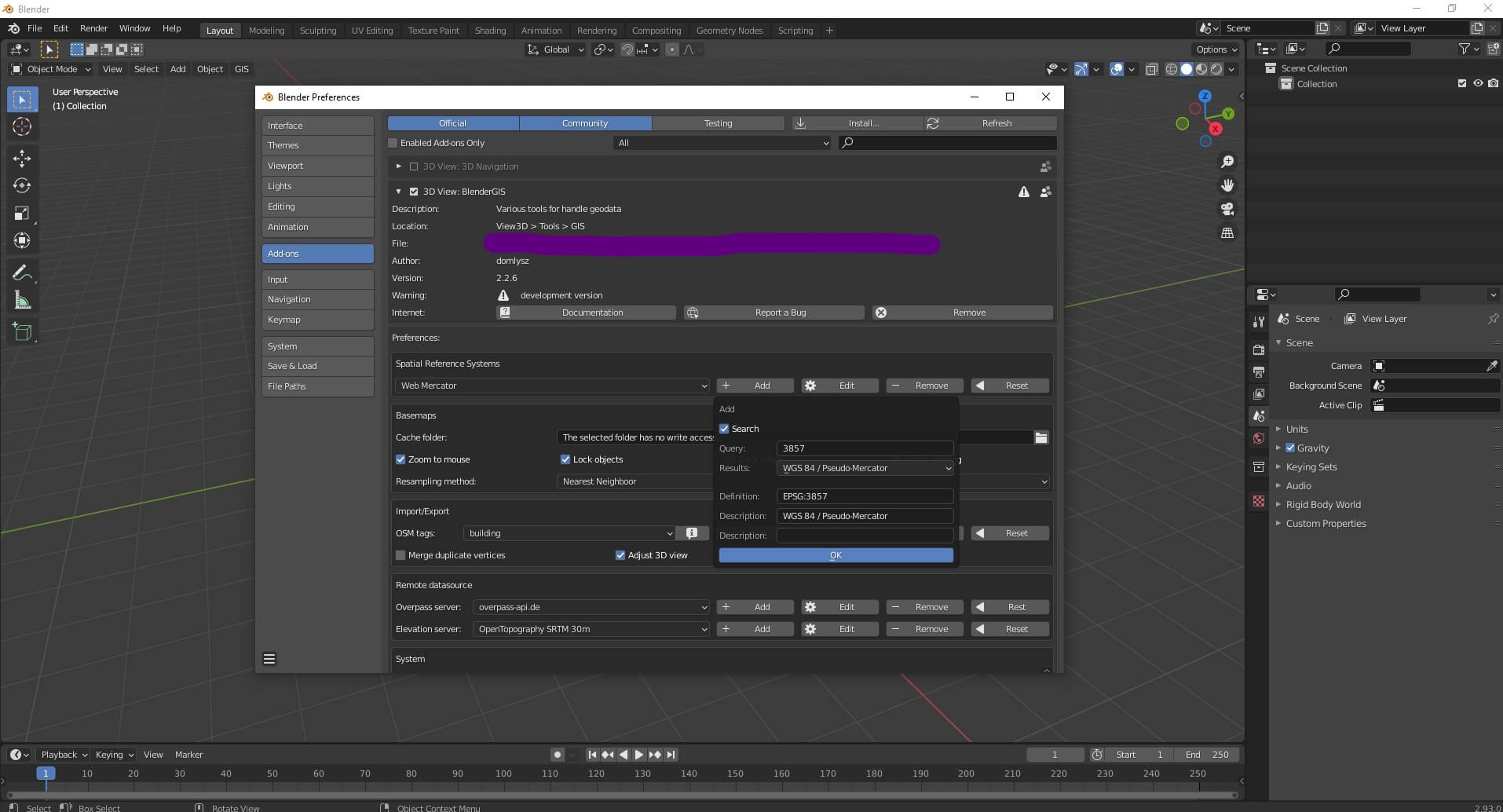
Always have the little tick icon next to the BlenderGIS. It means that the plugin is active. If click the arrow next to the check box, you access more settings. Here you can add new coordinate systems based on EPSG codes. After finishing the setup, you can close the “Blender Preferences” window. If there is a “GIS” option among the buttons in the top left corner of the model space (next to the “Object”), the installation was successful.
Sidenote: If you want to create a generalized model, based on blueprints, and you want to compare it to the results of your survey, you can do that in Blender too. However, this requires a lot of practicing.
BLENDERGIS IN ACTION
In the next chapter we take a look at how we can place reference points on models in Blender. Sadly, Blender is unable to work with such simple geometries as lines and points. But in BlenderGIS we have the opportunity to read points from the shapefile. To do this first we need to create a shapefile. It’s best to do this in QGIS. After that, we open the shapefile (containing geometries) with BlenderGIS and place it in the 3D space, fitted to the final model.
CREATING A SHAPEFILE
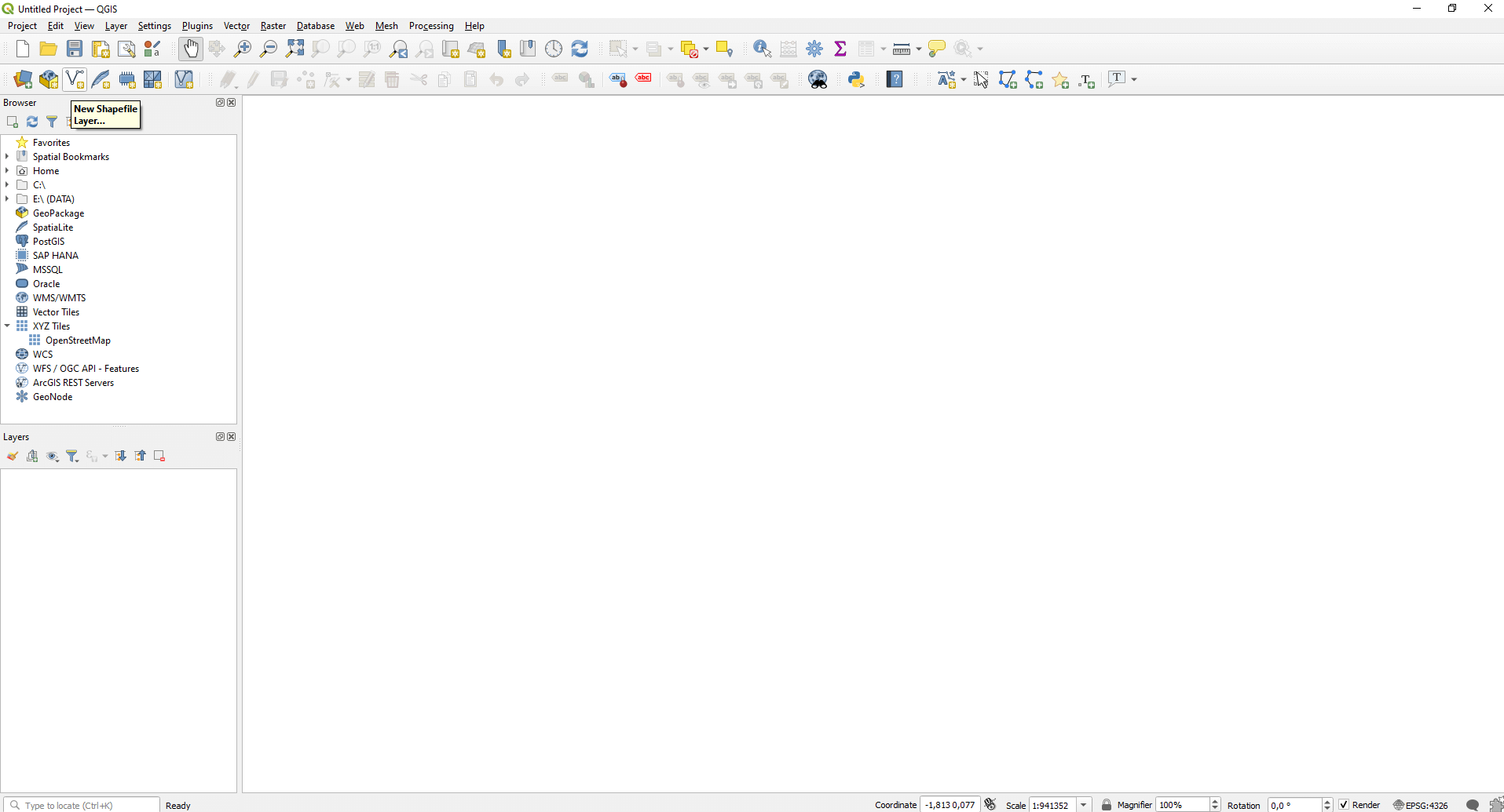
Open QGIS and click the “New Shapefile Layer…” button in the top menu bar.
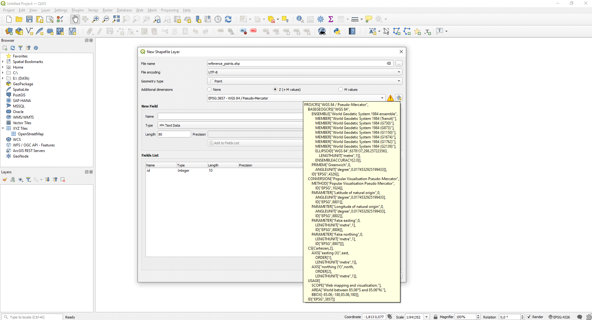
Create a shapefile with point geometry which has “Z (+M values)” dimension. And don’t forget to set the same coordinate system your models are made in. We don’t deal with attributes now. If you want to read more about shapefile creation I recommend the following article from us.
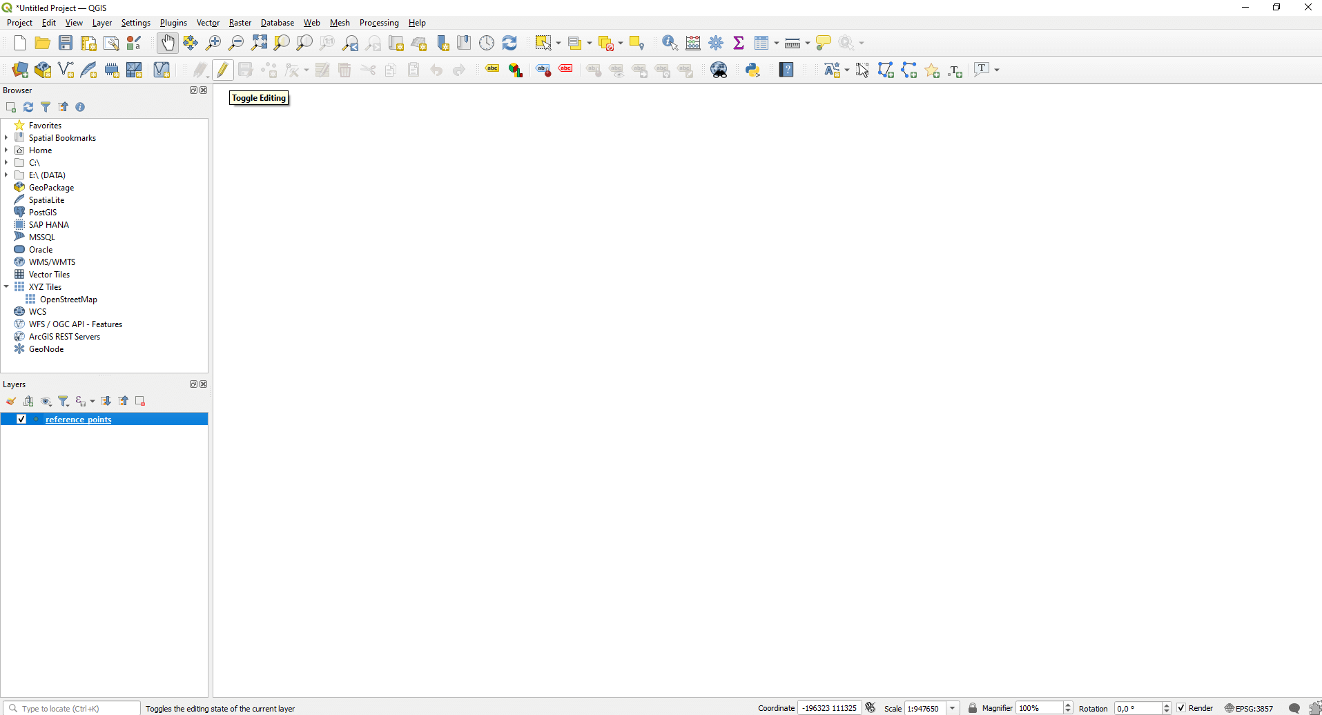
After the data file is created QGIS automatically adds it to the layer tree. I recommend placing a point near your building model. To do this, you need to activate editing on the layer. Select the new shapefile layer in the layer tree with left click and press the “Toggle Editing” pencil icon.
Now the “Add Point Feature” button becomes available, two buttons right from the pencil. Click on it, what could go wrong? 🙂 Now you can place your point geometry on the map. In this case you have two options: you may import a base map to be able to place the point, or you can give the location of the point with coordinates. You can import the base map with the “Browser” window above the layer. Click on the “OpenStreetMap” icon under the “XYZ Tiles” and the base map shows up immediately. You can zoom with the mouse scroll and you can place a point anywhere with the left mouse button (if your layer is selected in the layer tree). Finally, press the “OK”.
Don’t worry if your point doesn’t show up. Probably you made everything right. You just need to change the layer order in the “Layers” window, because right now the base map covers your point. Simply grab the layer of the point and pull it above the “OpenStreetMap” layer. The result shows right away. 🙂
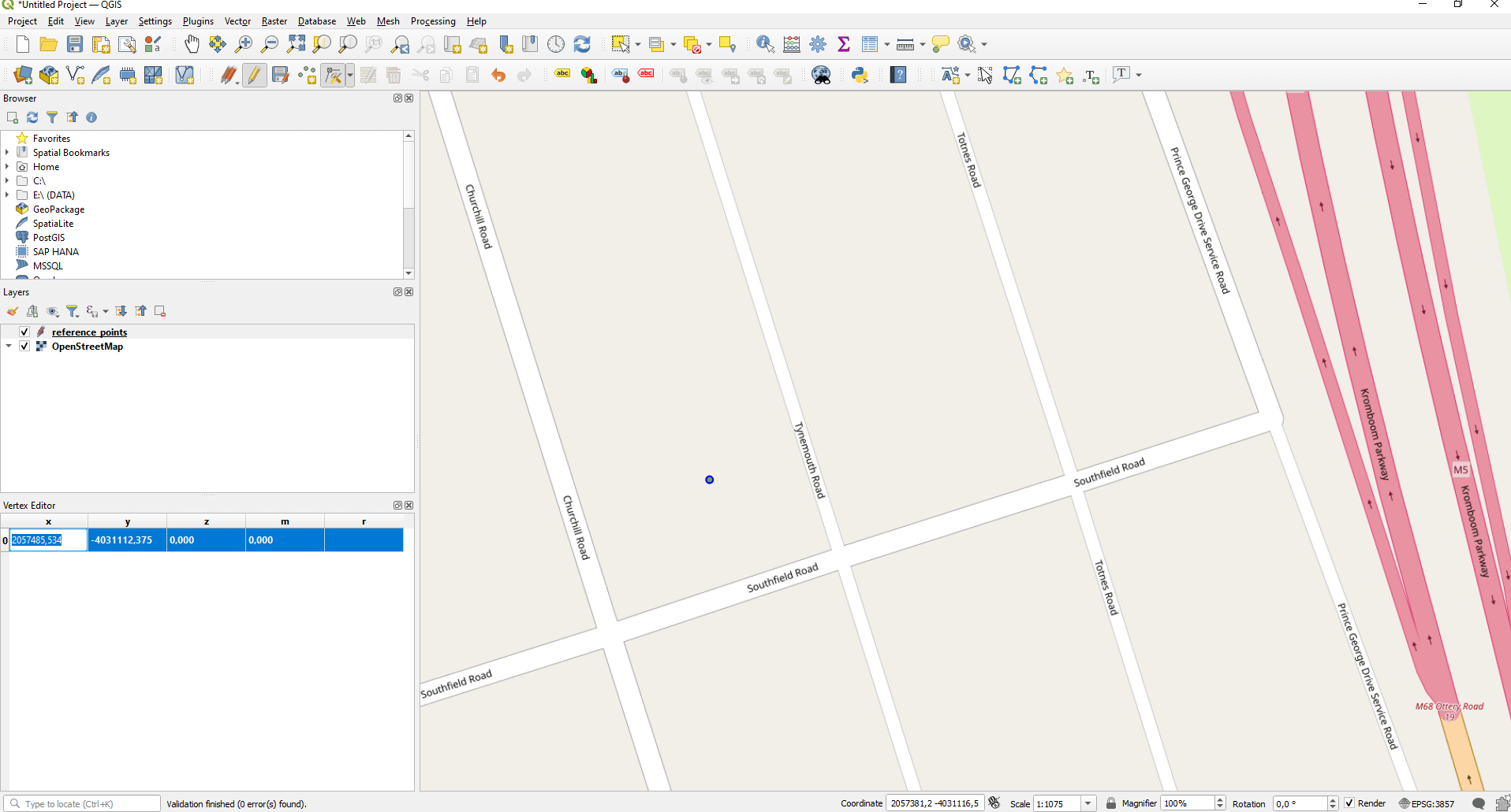
If your point is not in the right position, it’s enough to overwrite the coordinates. You can do that by clicking on the “Vertex Tool” which is right next to the “Add Point Feature” button.
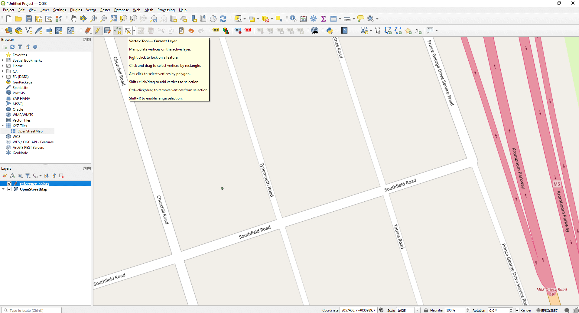
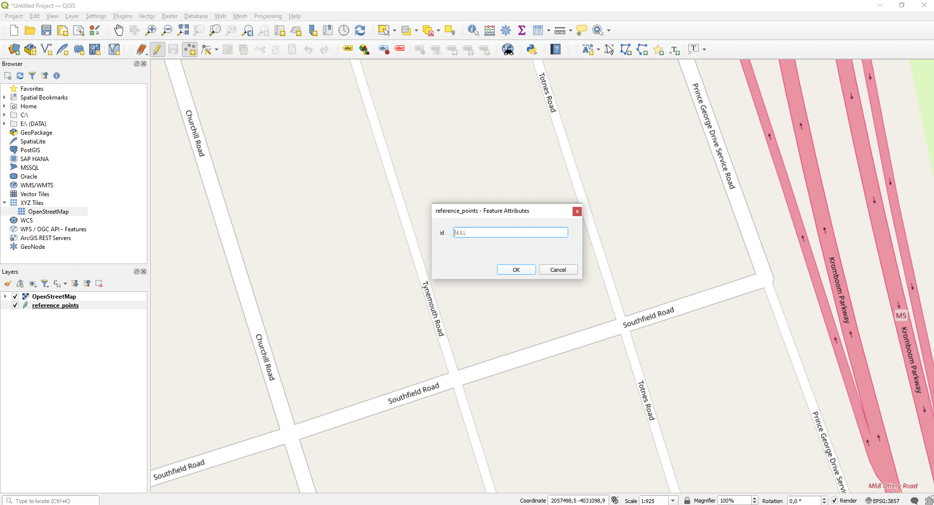
Now right click to your point on the map. A window will appear in the bottom left corner where you can set the X, Y, Z coordinates.
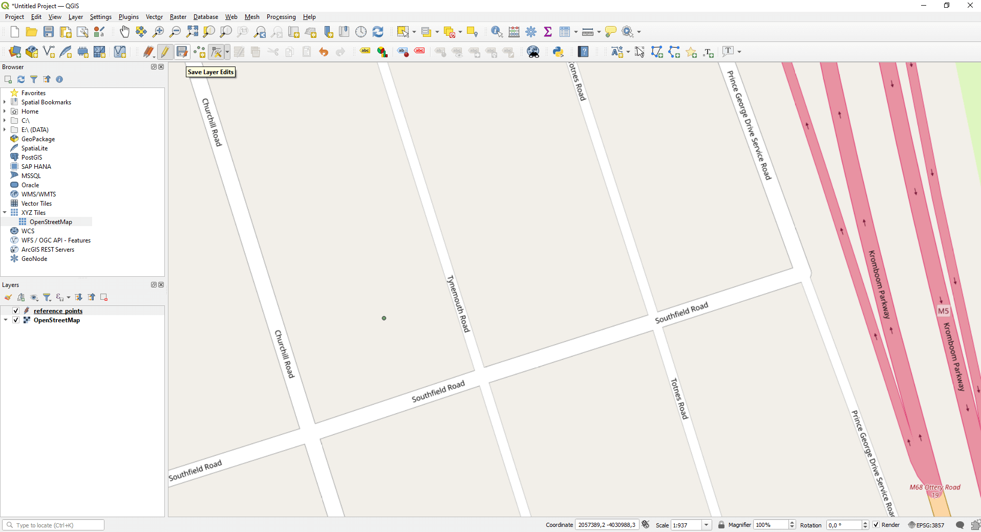
After finishing, save the layer with the “Save Layer Edits” button in the top menu bar. Close the editing process with choosing the “Toggle Editing” button.
PLACING POINTS IN BLENDER
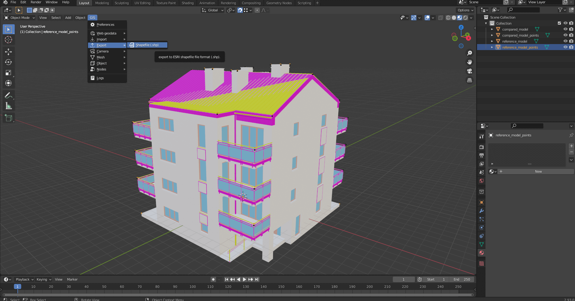
Let’s get back to Blender! Thanks to BlenderGIS now we have a “GIS” button in the menu of the model space. Click on this with the left mouse button and under “Import” choose “Shapefile (.shp)”.
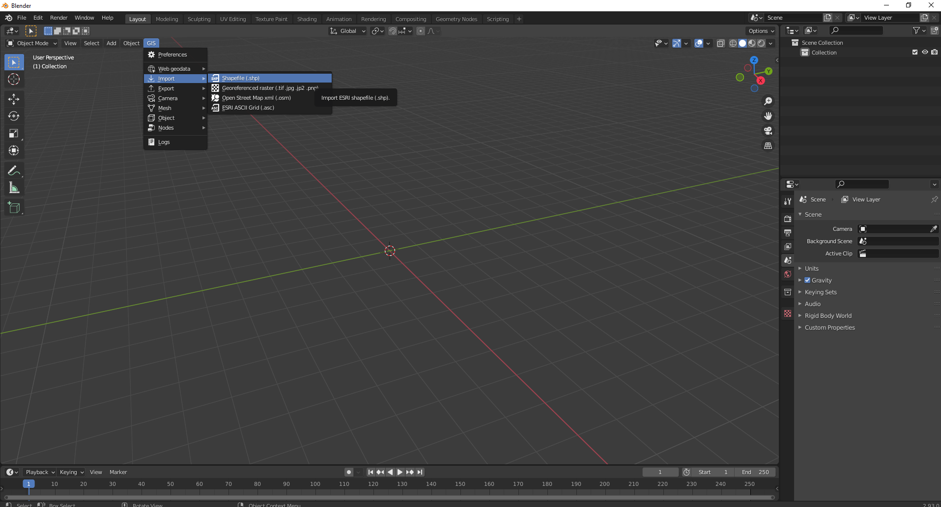
Browse the previously created shapefile and add it to the model space. For now, we only clone the imported file and rename the layers. You can do that by selecting the layer with the left mouse button in the top right window and pressing “Ctrl+C” and “Ctrl+V”. A new layer appeared with the same name as the imported shapefile, except that this ends with “001”.
Rename the layers in order to always know which one applies to the starting and the end result. Do that by double clicking on the name of the layer.
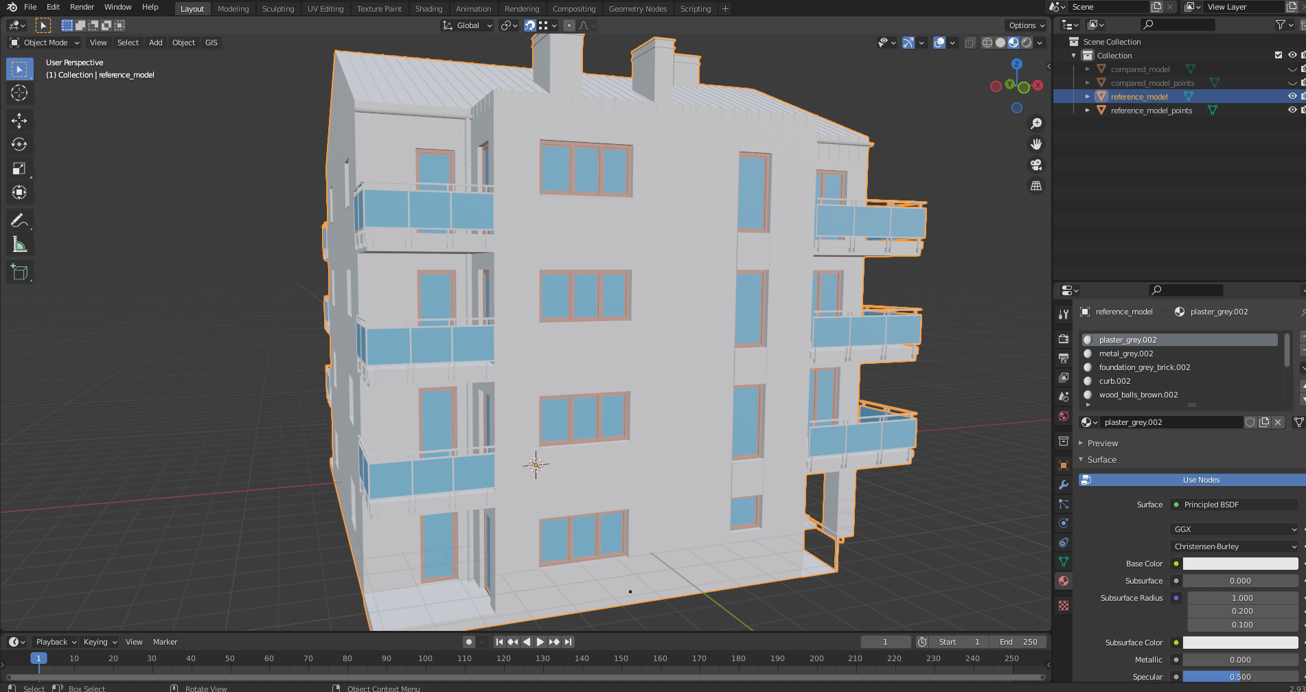
After all this we import the models. In the “File” menu (which is in the left corner) you choose the “Import” option and browse for your model. Always take care to set the “Forward” value to “X Forward” and the “Up” value to “Z Up” in the “Transform” menu. Do this process for each model. After importing the models it again can be useful to rename the layers. If a layer bothers you, you can “temporarily) hide it by clicking on the small eye icon in the layer tree next to the layer.
Sidenote: You can place reference points on point clouds in Blender, but for that you’ll need another plugin, called Point Cloud Visualizer. Watch this video to learn how to use point clouds in Blender. If you decide to use this method, prepare yourself that it will be much harder to adapt reference points to the point cloud.
Let’s jump right into the placing of the points. Firstly choose the location of the potential reference points on the model. Do this with the same point of view as you would do when georeferencing. Concentrate on the clearly visible points that both models have. These points can be corners and intersection points.
In Blender you can turn the view around by moving the mouse while holding the mouse scroll. If you hold the “Shift” button too, you can drag the camera. Of course you can zoom in and out with the mouse scroll.
Select the shapefile layer containing the point geometries in the layer tree. Activate the “Snap function” before we start to move the points. This will make our point to adapt to the model’s surface and vertices which makes it easier to move it in 3D. The magnet icon of “Snap” function can be found in the top center of the model space. The function is active when the button’s background is blue. Select “Vertex” option on the right side of the magnet. This means your reference point will adapt to the model’s vertices.
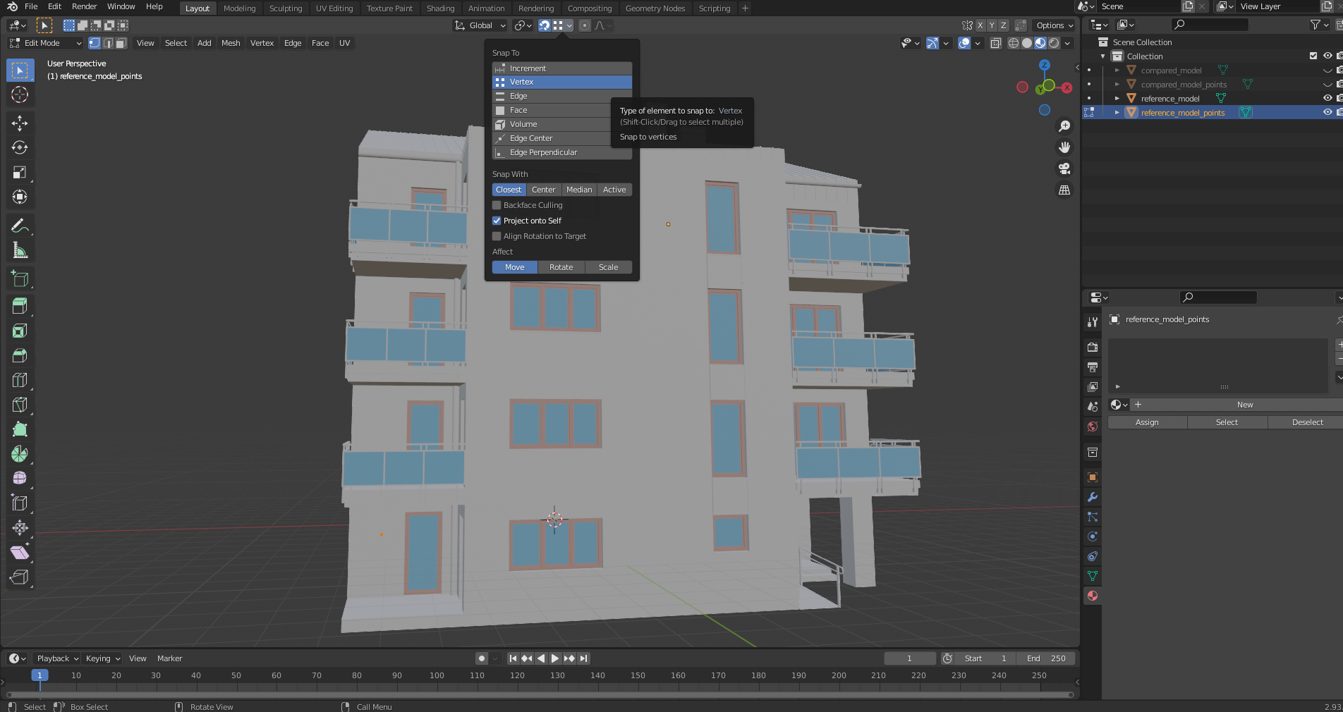
Move the cursor above your point and press the “G” key to start moving the point.
Sidenote: At this stage it’s worth it to save the Blender project regularly to avoid any data loss due to an unexpected freeze or crash of the program. The project file, which is in “blend” format can be saved under the “File” menu. The Blender files will contain the displayed data files on their own so you won’t need them as an external data source.
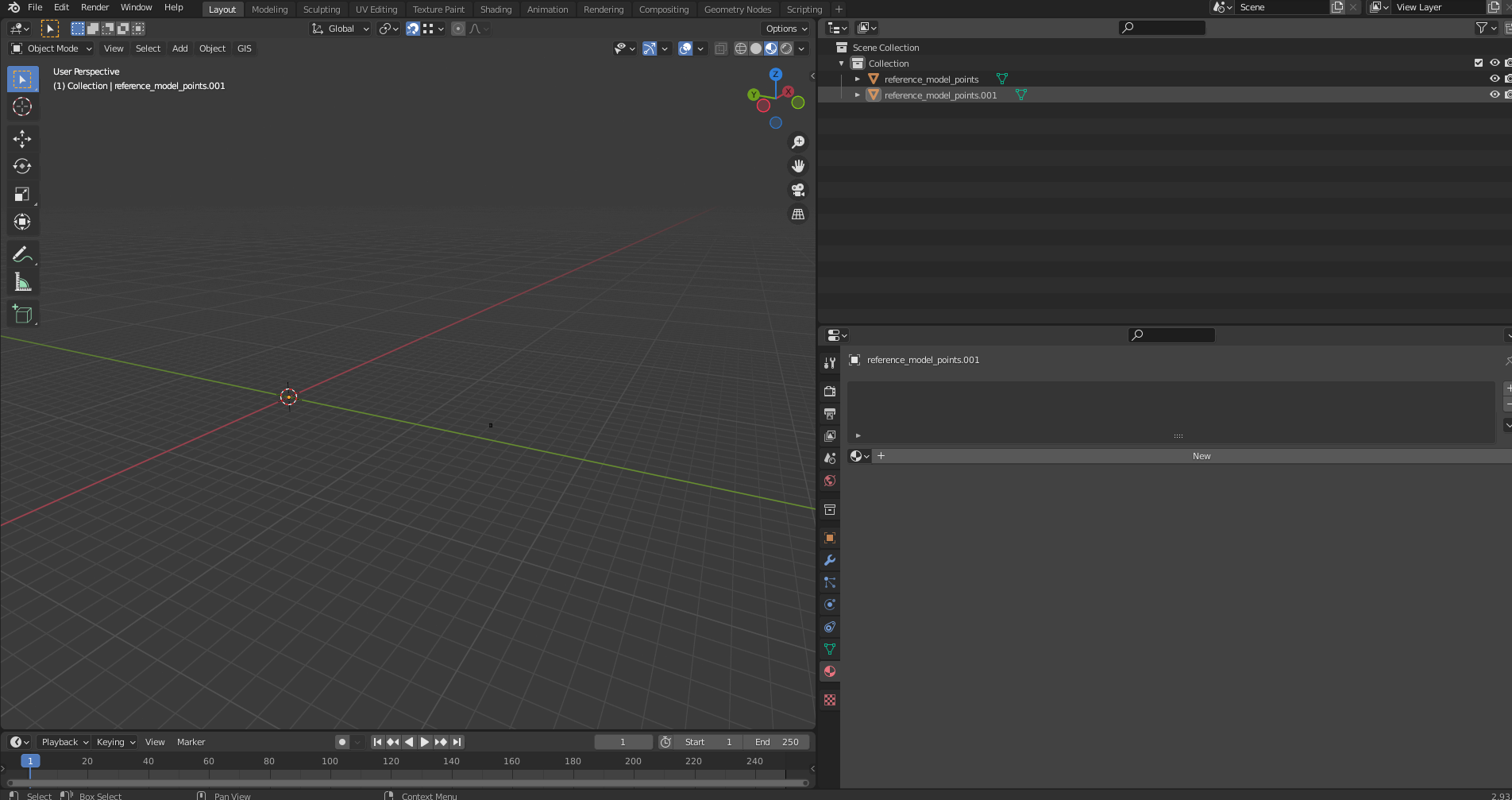
If you’ve successfully placed a reference point, press “Ctrl+C” and “Ctrl+V” to copy the layer. As before, move the new point to the selected place of the next reference point and repeat these steps until you reach the number of points you deem necessary. Once you’re done with placing new points, merge the layers into one. Select all the reference point layers with “Ctrl + Left mouse button” or “Shift + Left mouse button”. Move the cursor to the model space and press the “F3” key, then to the search field type “Join”. By taking the first option Blender will merge your layers into one.
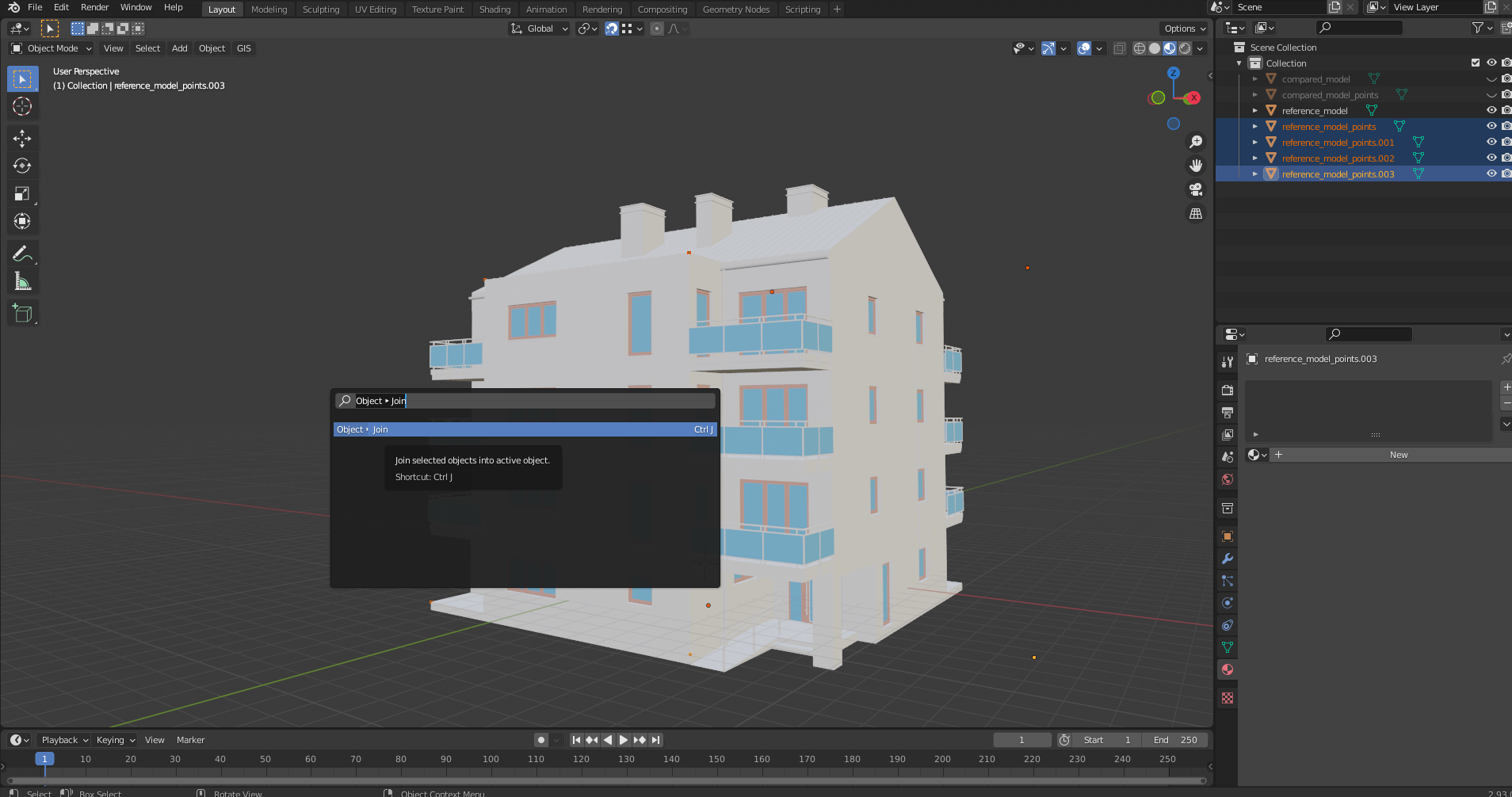
Do this process regarding the other model too. If you made everything as I told you, there should be 4 layers in the layer tree at the end of the process:
- Starting state model
- End state model
- Reference points of starting state model
- Reference points of end state model
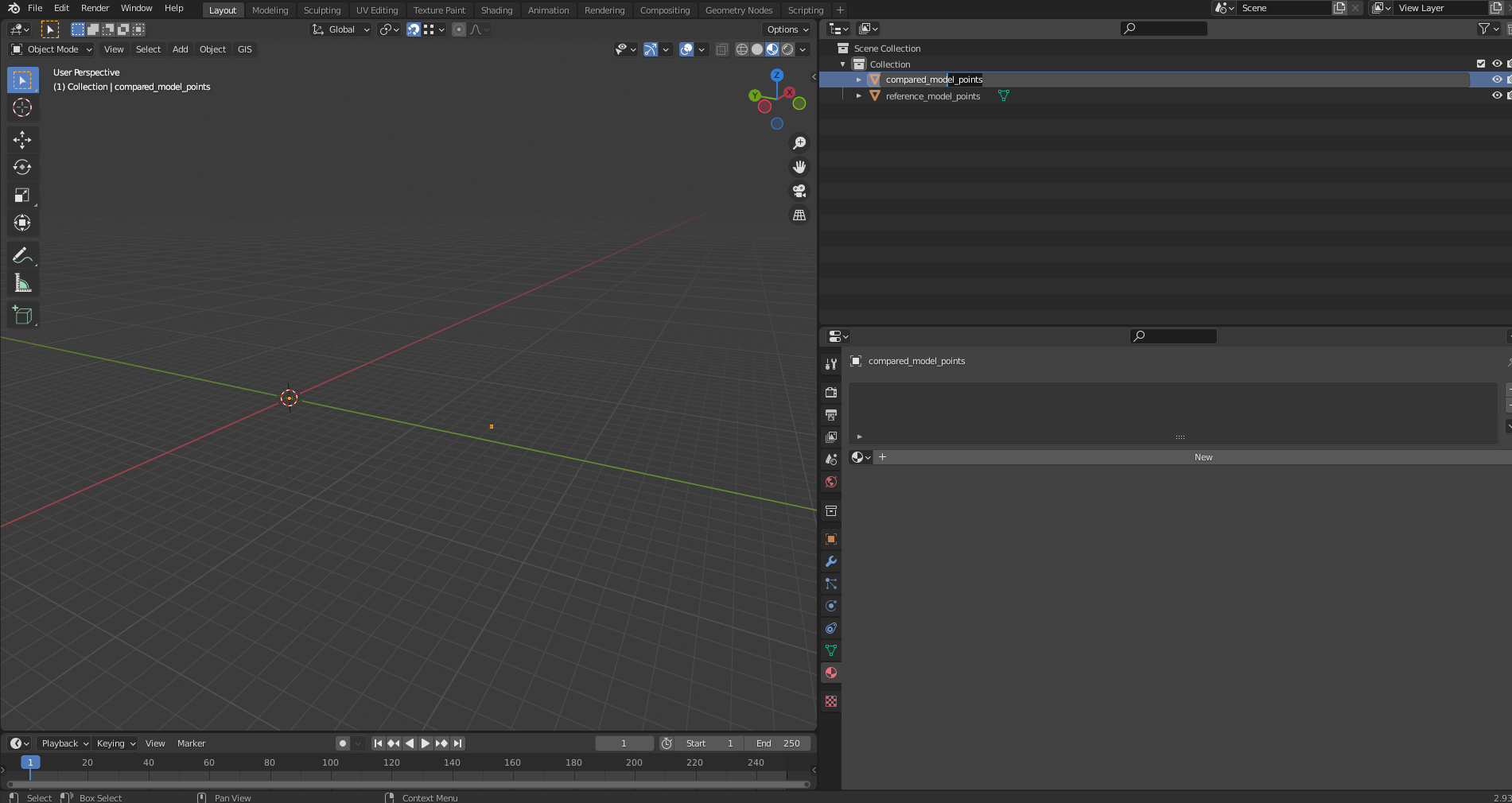
The last thing left is exporting the reference points which we will make the distance measuring on. Select one of the point layers in the layer tree. Now click on the “GIS” button and pick the “Export” option, then the “Shapefile (.shp) option. Of course you need to export the other point layer too.
DATA ANALYSIS
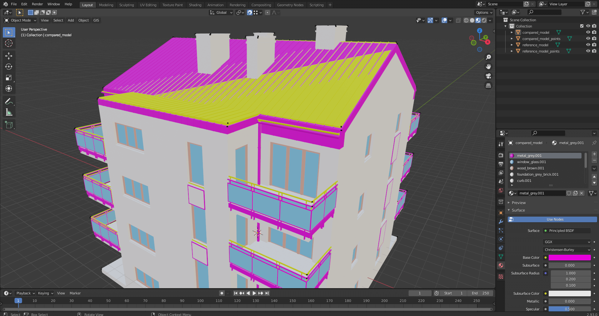
In this section you will get the first results that visualize the degree of displacements (distances). We do this process in CloudCompare. As I mentioned, we will see what results we get if we analyze reference points in case of distorted spatial location. Also we take a look at the result if we only analyze surfaces while the spatial parts are changing.
Sidenote: In CloudCompare it’s possible to snap two models to each other (georeference). You can do this manually or automatically. In both cases the first step is to select the models from the layer tree. For the automatic method you click on the „Fine Registration (ICP)” icon. There is a function called “Auto align clouds” but I don’t recommend it, because it has a lot of bugs. The manual method is technically a georeferencing process, which you can do using the “Align (point pairs picking)”
tool in the menu bar.
MEASURING REFERENCE POINTS
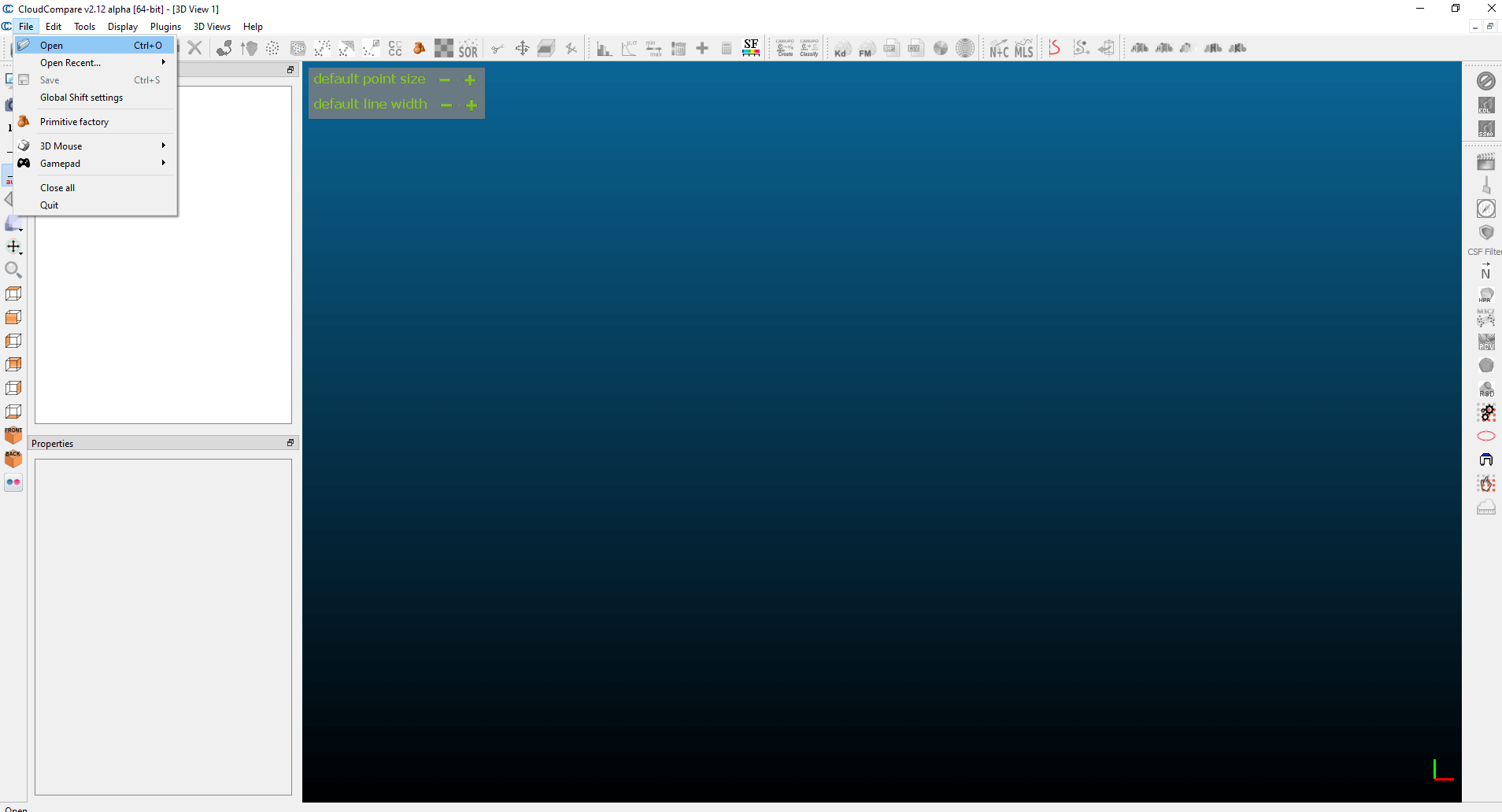
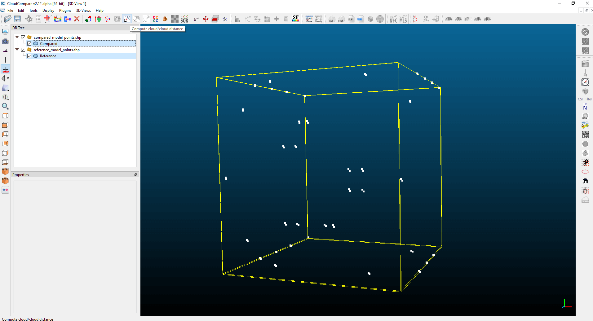
Open CloudCompare. Under the “File” menu click on “Open” to import the exported shapefiles from Blender.
They appear as if they were point clouds and this is perfect for us. Rename both layers called “Cloud #1” with double clicking on its name. Select the layers by holding the “Ctrl” key. Then choose the “Compute cloud/cloud distance” function.
Choose the file which represents the starting state (“Reference”) and the end state (“Compared”).
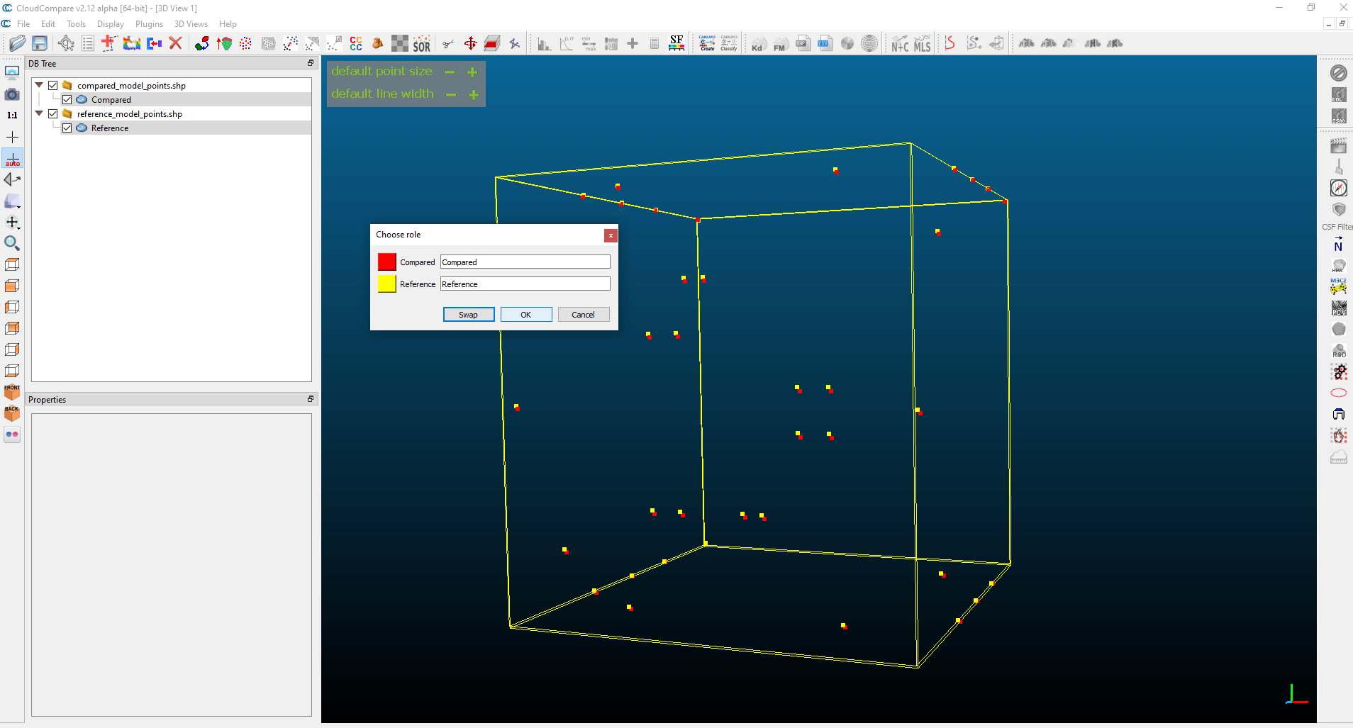
In the window that appeared you can set the parameters of the function. It’s important to tick the “split X, Y and Z components”. This will cause CloudCompare to separately calculate the measured distances along the X, Y and Z axis and they will be available as attributes. I won’t ruin the joke, but we will use these later.
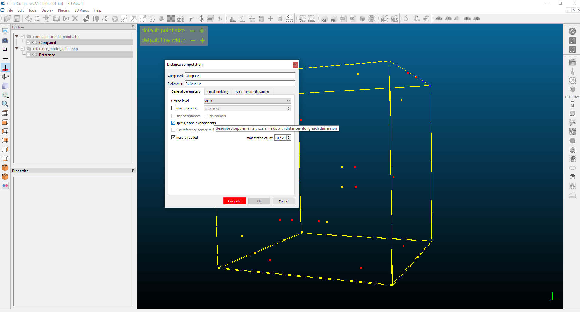
Click on the unmistakably red “Compute” button and then click on “OK”. You might think that all we did was coloring points, but this can’t deceive experienced GIS experts like us. 🙂 Select the “Compared” layer and press the “Shift+C” combination. A legend appeared on the right which shows the 3D distances (obviously in the same metric as you’ve been using). By selecting the layer, a lot of setting possibilities become available in the “Properties” window, under the layer tree. For example, the size of the displayed points, color scale, and the setting of minimum and maximum values.
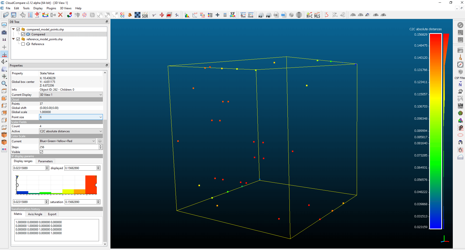
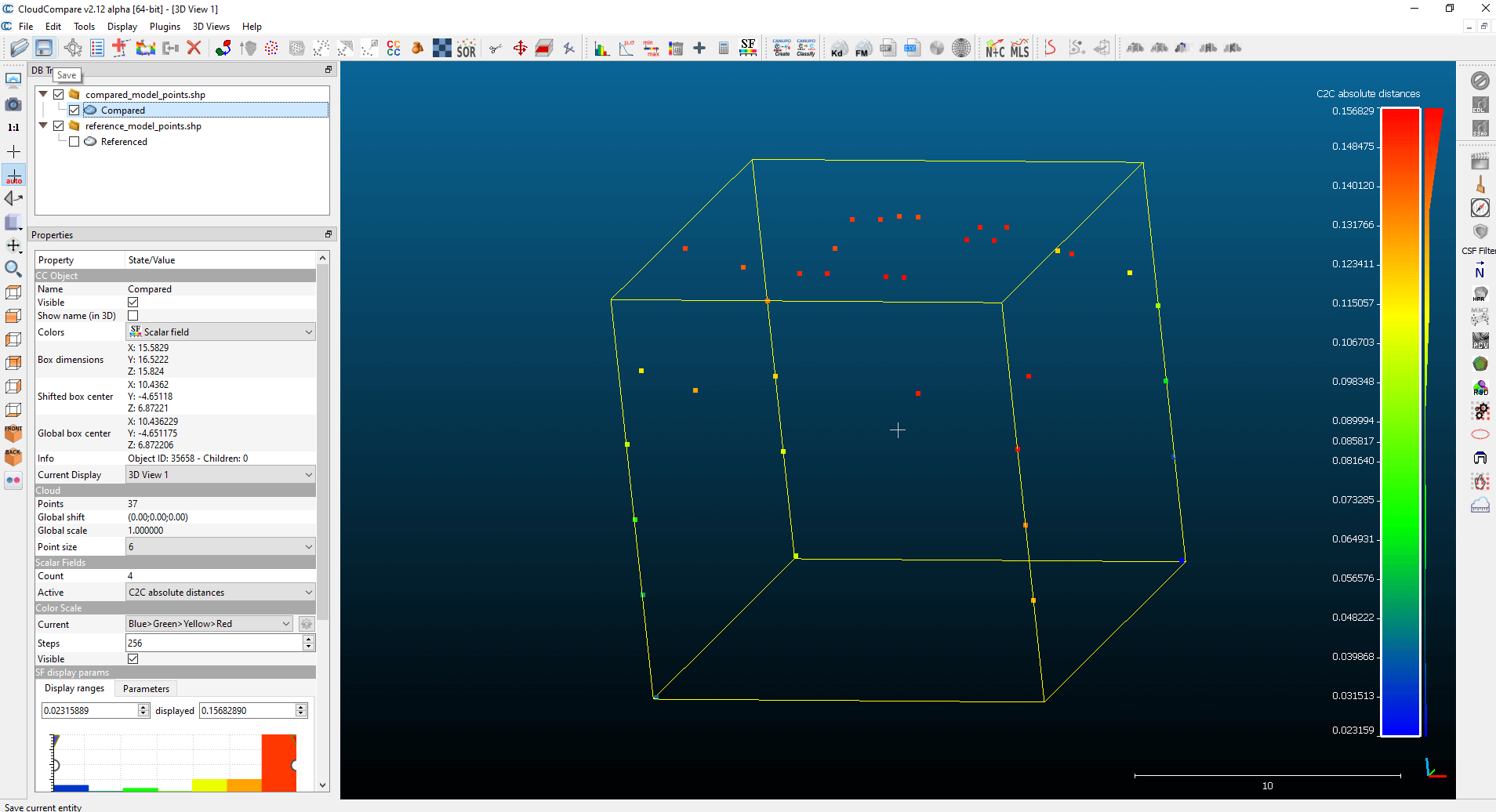
Now export the points with the result of the distance measuring. Select the “Compared” layer and press the blue floppy disk shaped “Save” button.
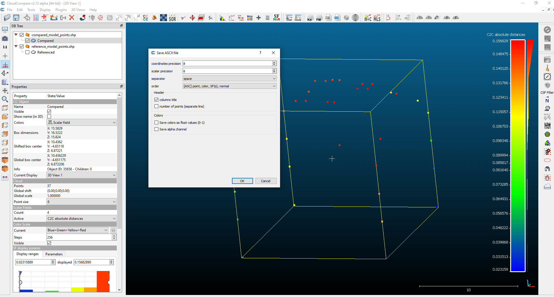
Choose the “ASCII cloud” option. To the end of the file’s name type “.txt”. If you don’t do this the CloudCompare will create a file without extension. Finally, set the column names to be visible, by ticking “columns title” in the “Header” box. Press “OK” and we’re finished.
ANALYZING SURFACES
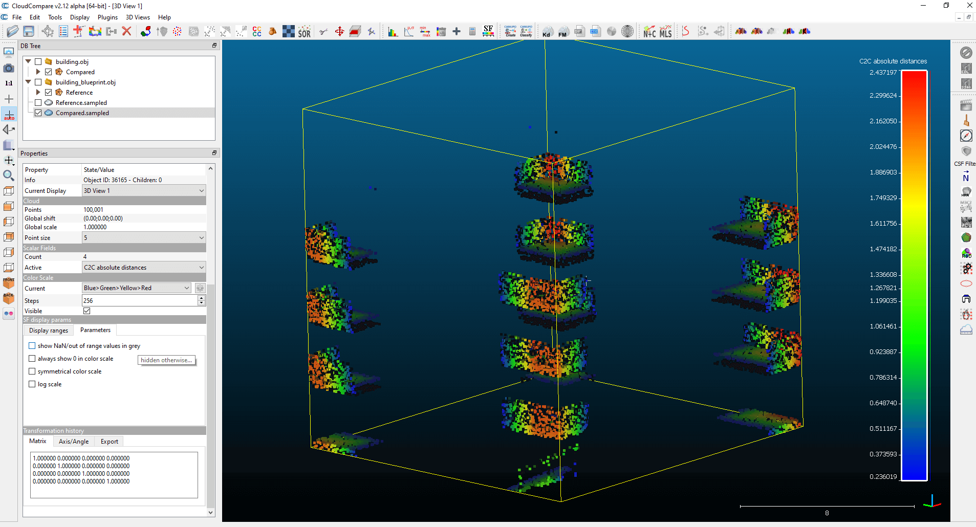
In this chapter we will see what results we get if we don’t have to bother with placing reference points, we only have to compare the two models. Start CloudCompare and open the starting and the reference models. You can open both mesh models and point clouds. If you work with a mesh file, first you need to convert it into a point cloud. Select the layer, then use the “Sample points on mesh” function.
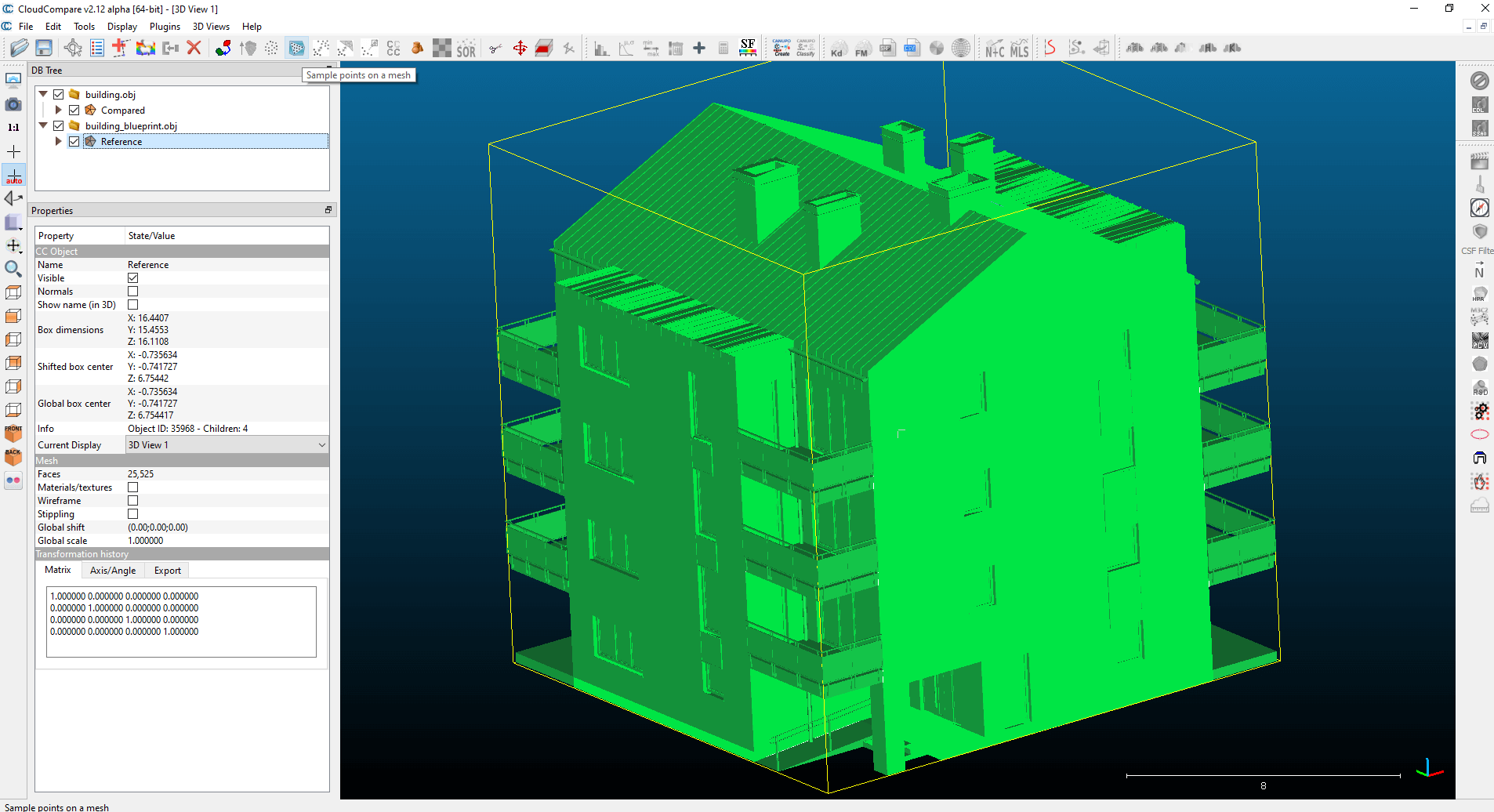
Set how many points you want from the mesh and press “OK”. Select the new point cloud layers and run the “Compute cloud/cloud distance” functions as shown before. In this version the result will be more conspicuous because of the higher number of data points. It’s clearly visible that while the reference building model did not have balconies, the result model has them. This difference is easily noticeable.
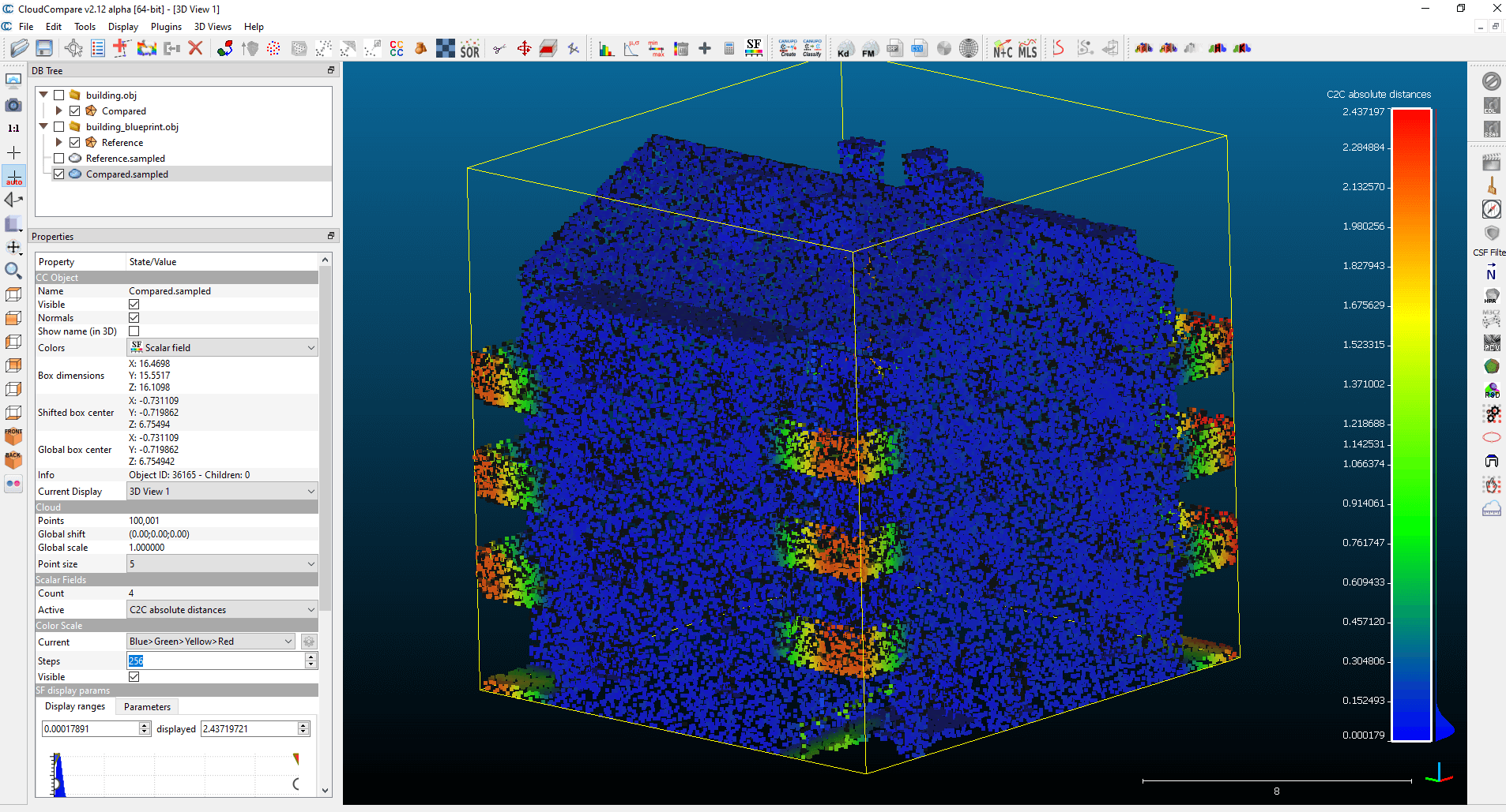
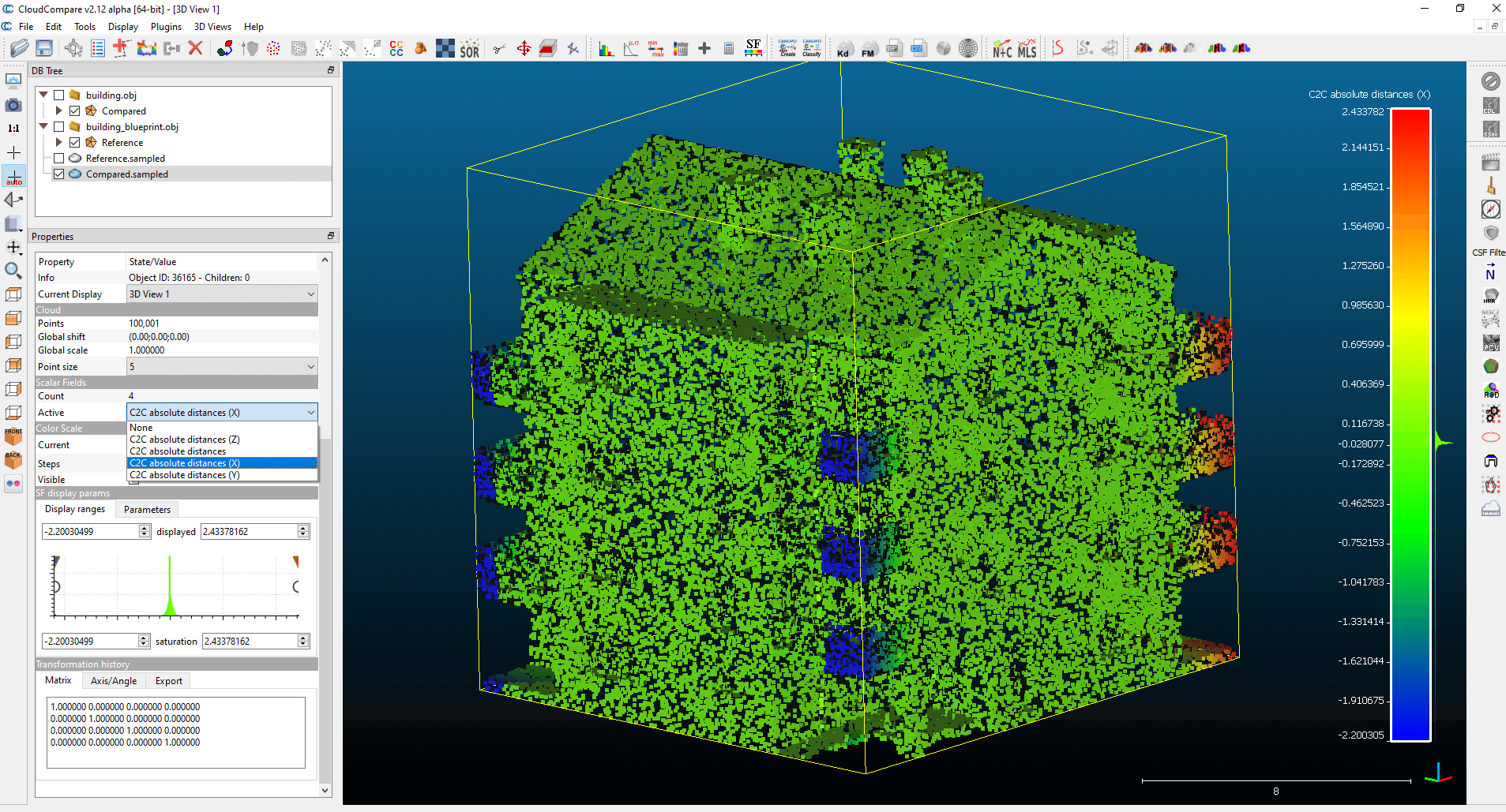
Under the properties of the layer, you can discover the many ways you can display the result. For example, you can set the distances to be shown only along the X, Y or Z axis.
Furthermore, under the “SF display params” block you can set the interval you want to be contemplating. The inactive sections will appear in gray.
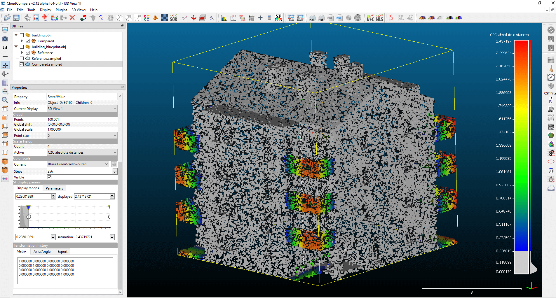
If you would hide the gray parts, you can do it under the “Parameters” tab by turning off the “show NaN/out of range values in grey” option.
If you would save this display there is one step left. You need to de facto filter the data (the previously presented method was just a displaying technique). Open the “Edit” menu and choose the “Scalar fields” submenu, then the “Filter By Value” option.
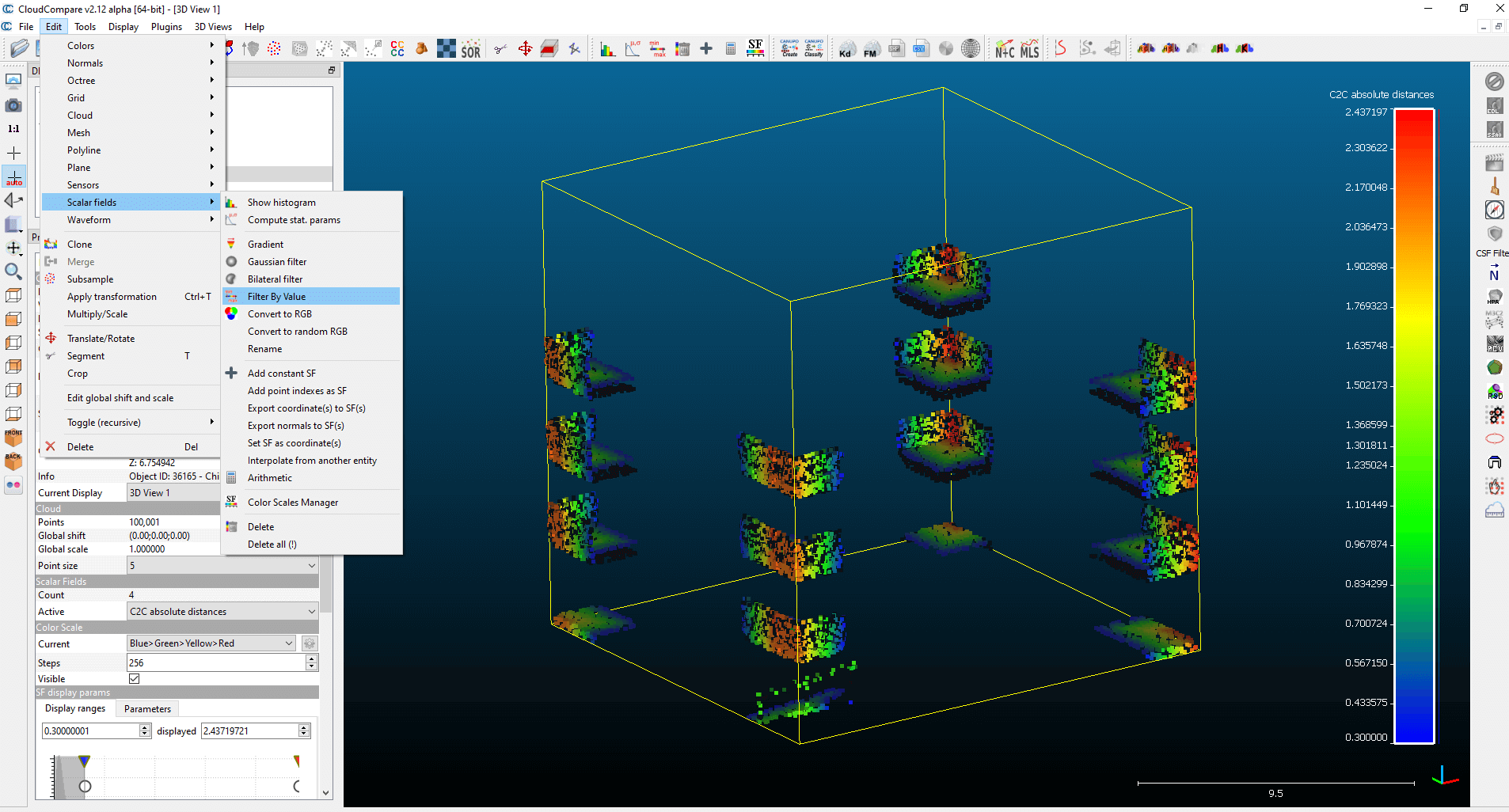
Here you can again set the minimum and maximum values of the filter. You have the chance to split the data table, based on values that are in, or out of the interval. In addition, with the “Export” button you can export the filtered interval. So that’s what we’re going to do.
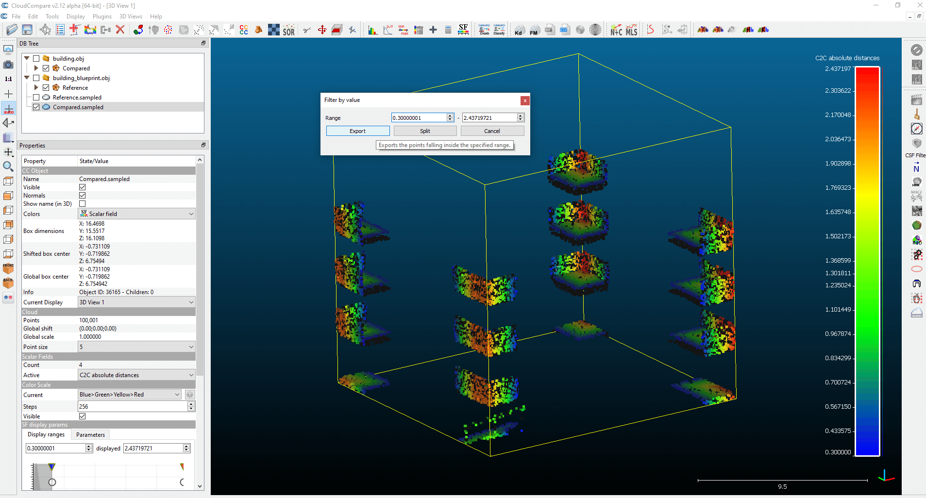
A new layer appeared, containing only the data from the specified range. The layer ends with “extract”. You can export these as simple ASCII files, as I’ve shown in the previous chapter.
EVALUATION AND DISPLAY
So far, we haven’t necessarily used only GIS functions, but from now on it will be only them. Through the evaluation we will use QGIS. You may ask: if we have the distance in CloudCompare, why do we have to do anything with QGIS? Well, this process will determine the tilt and bearing of every single measured distance. If you are aware of these data, you can determine on a statistical basis the direction and extent of the building being examined.
Sidenote: It’s worth mentioning the philosophy of all the GIS software (including QGIS). There are different data sources like shapefiles, data tables from databases, WFS or WMS connections etc. And apart from those there is the QGIS project file, which you can save in “qgz” or “qgs” formats. The project file does not save the data itself, only their path and the used settings (for example: filters, style elements, layer order). Because of that, always keep your data available and always be aware where you store them. If you would use those data tables in an external software, export the layer instead of trying to save the QGIS project file.
REFERENCE POINTS
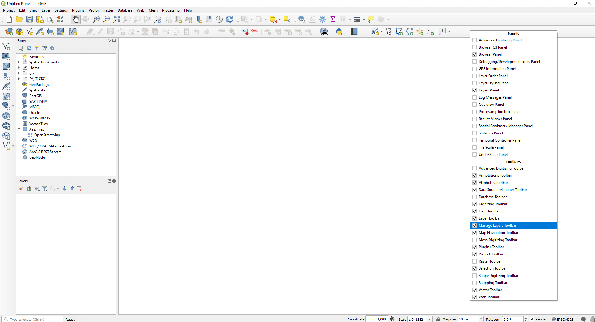
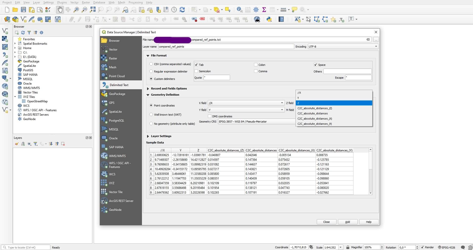
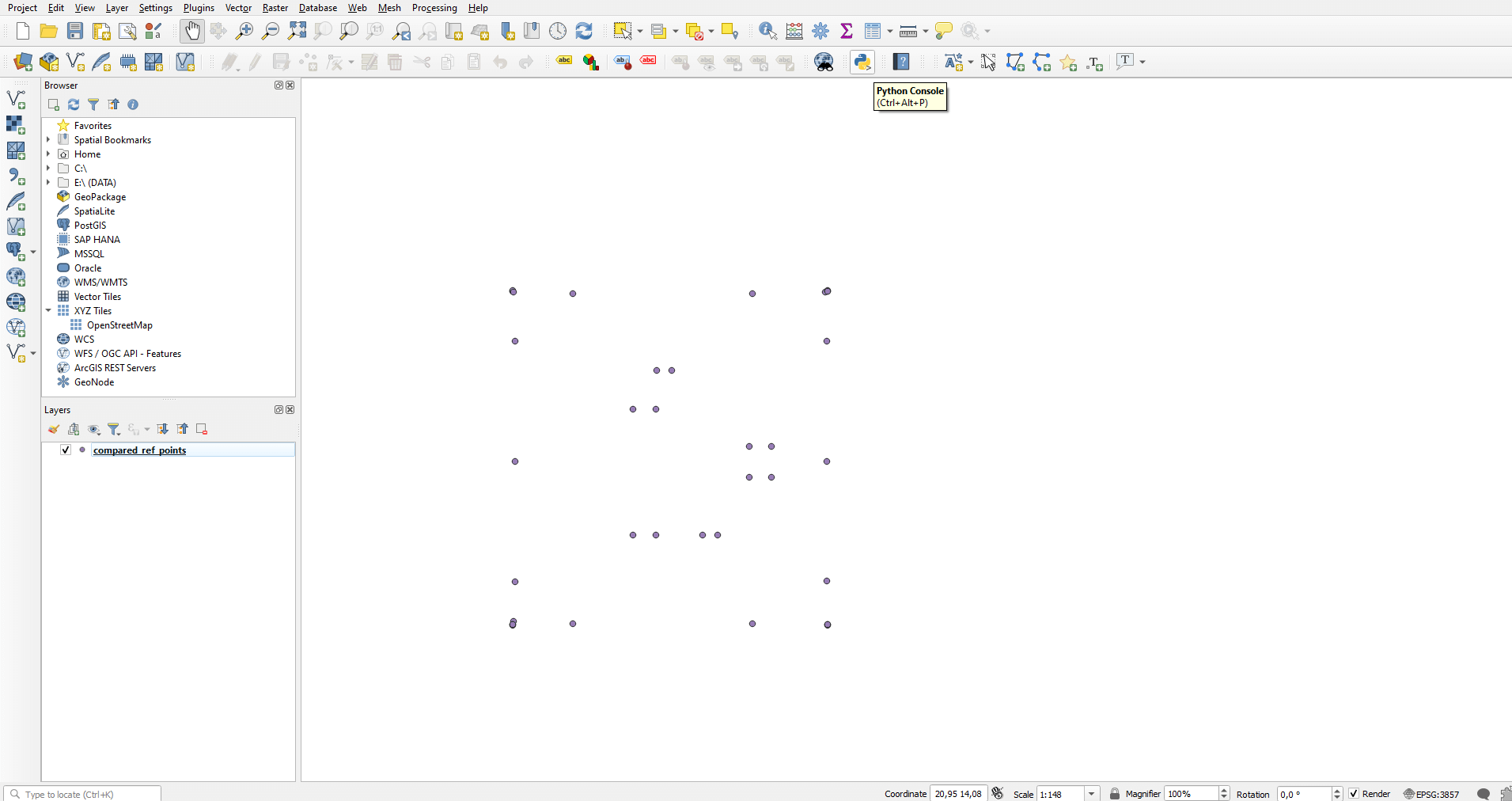
In this section we will import the “txt” file from “CloudCompare” as a shapefile. Start QGIS and create an empty project. Click on the top menu bar with the right mouse button and activate the “Manage Layer Toolbar”. New icons will appear in the sidebar next to the “Browser”.
Pick “Add Delimited Text Layer” from the sidebar. Look for a comma shaped button. Browse the text file and set the character which separates the columns. Finally, add the columns containing the X, Y, Z coordinates and set the coordinate system too if needed. Then click on the “Add” button and close the window.
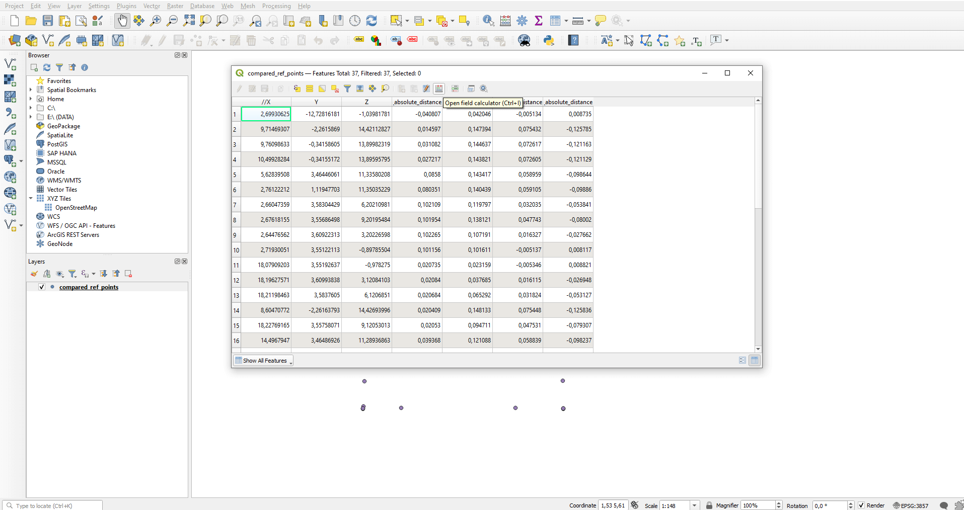
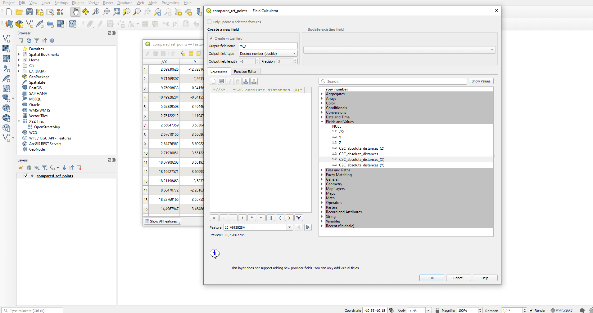
Congratulations, we have created the already existing points in QGIS! 🙂 Okay, in fact these are much cooler points, because they contain distance data. However, for calculating the direction of inclination and the angle of inclination we need to create 3D lines. The starting points of the lines are already there, because we drew the points based on them. However, we don’t know the coordinates of the endpoint. Let’s calculate them! Right click to the layer and open the attribute table. Open the field calculator tool.
Create a column and name it “to_X”. You could call the column whatever you want to, all you need to keep in mind is that it will mean the X coordinate of the endpoint of the 3D line. Set the value of the “Output field type” dropdown list to “Decimal number (double)”. This means that the columns can contain fractions. After that you need to type in the following formula:
"//X" - "C2C_absolute_distances_(X)"
“//X” is the name of the column that contains the X coordinates, while “C2C_absolute_distances_(X)” is the column for the measured X distance. As an alternative, you can add these values under the “Fields and Values” point in the left search bar.
Do the same for the Y and Z coordinates, like that:
"Z" - "C2C_absolute_distances_(Z)"
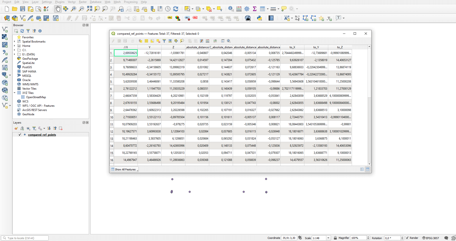
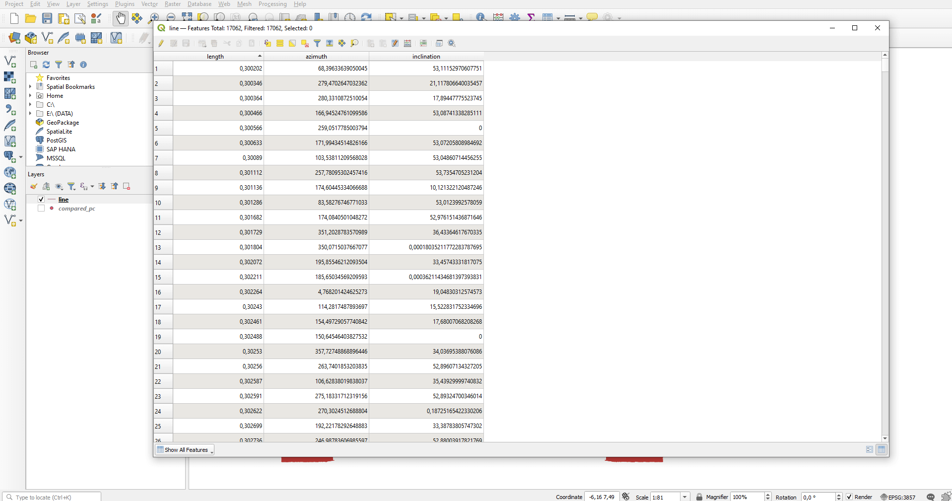
At the end you need to get 3 columns. Once you’re ready you should see something like that:
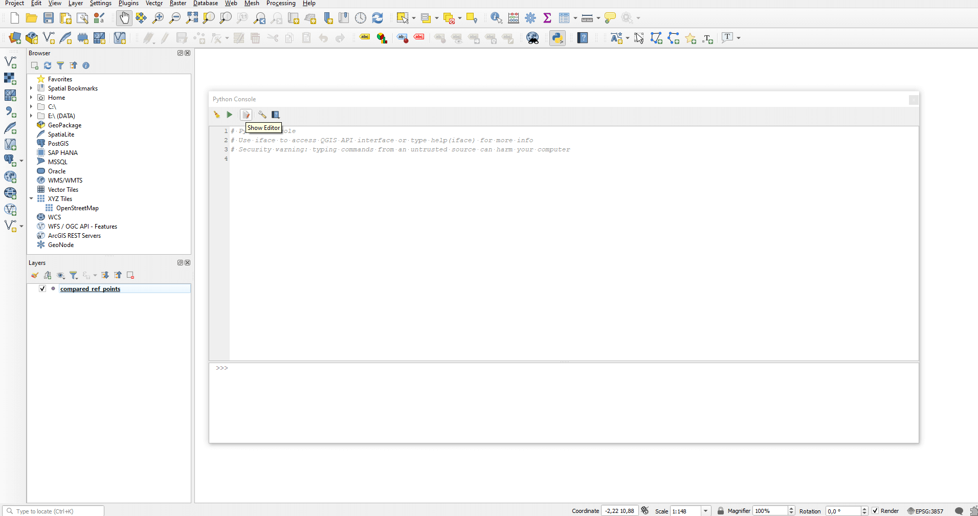
And here comes the part when half of the readers will exit the page. We will write Python scripts. I kindly ask you to wait until the end. I wrote the code so you have almost nothing to do with it. Open the “Python Console”. It’s in the top menu bar, marked with a blue and yellow snake icon. Well, you could think: snakes and coding, good things can’t come from this point. Nothing “good”, only 3D lines! 🙂
A rather ominous picture greets the user: almost no buttons, only text fields and numbered lines. Click on the “Show Editor” button:
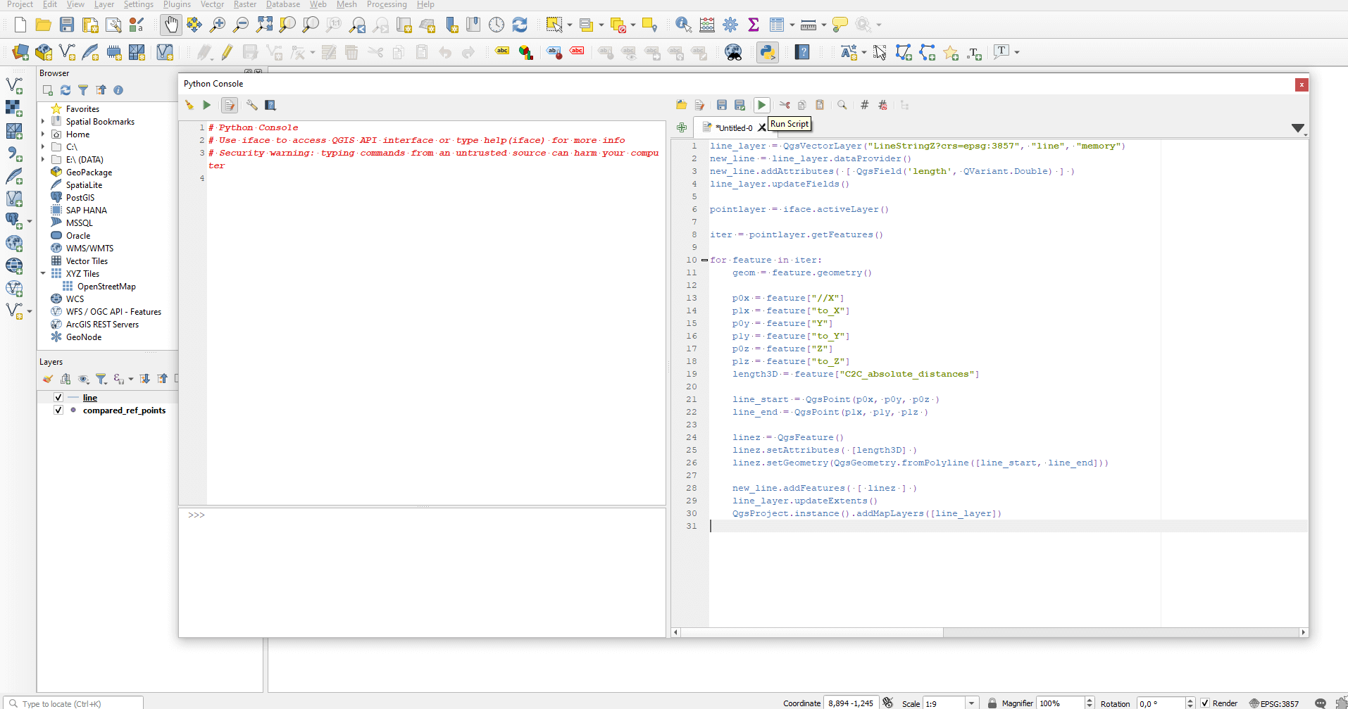
Paste this code into the field on the right:
line_layer = QgsVectorLayer('LineStringZ?crs=epsg:3857', 'line', 'memory')
new_line = line_layer.dataProvider()
new_line.addAttributes( [ QgsField('length', QVariant.Double) ] )
line_layer.updateFields()

pointlayer = iface.activeLayer()

iter = pointlayer.getFeatures()

for feature in iter:
    geom = feature.geometry()

    p0x = feature["//X"]
    p1x = feature["to_X"]
    p0y = feature["Y"]
    p1y = feature["to_Y"]
    p0z = feature["Z"]
    p1z = feature["to_Z"]
    length3D = feature["C2C_absolute_distances"]

    line_start = QgsPoint(p0x, p0y, p0z )
    line_end = QgsPoint(p1x, p1y, p1z )

    linez = QgsFeature()
    linez.setAttributes( [length3D] )
    linez.setGeometry(QgsGeometry.fromPolyline([line_start, line_end]))

    new_line.addFeatures( [ linez ] )
    line_layer.updateExtents()
    QgsProject.instance().addMapLayers([line_layer])
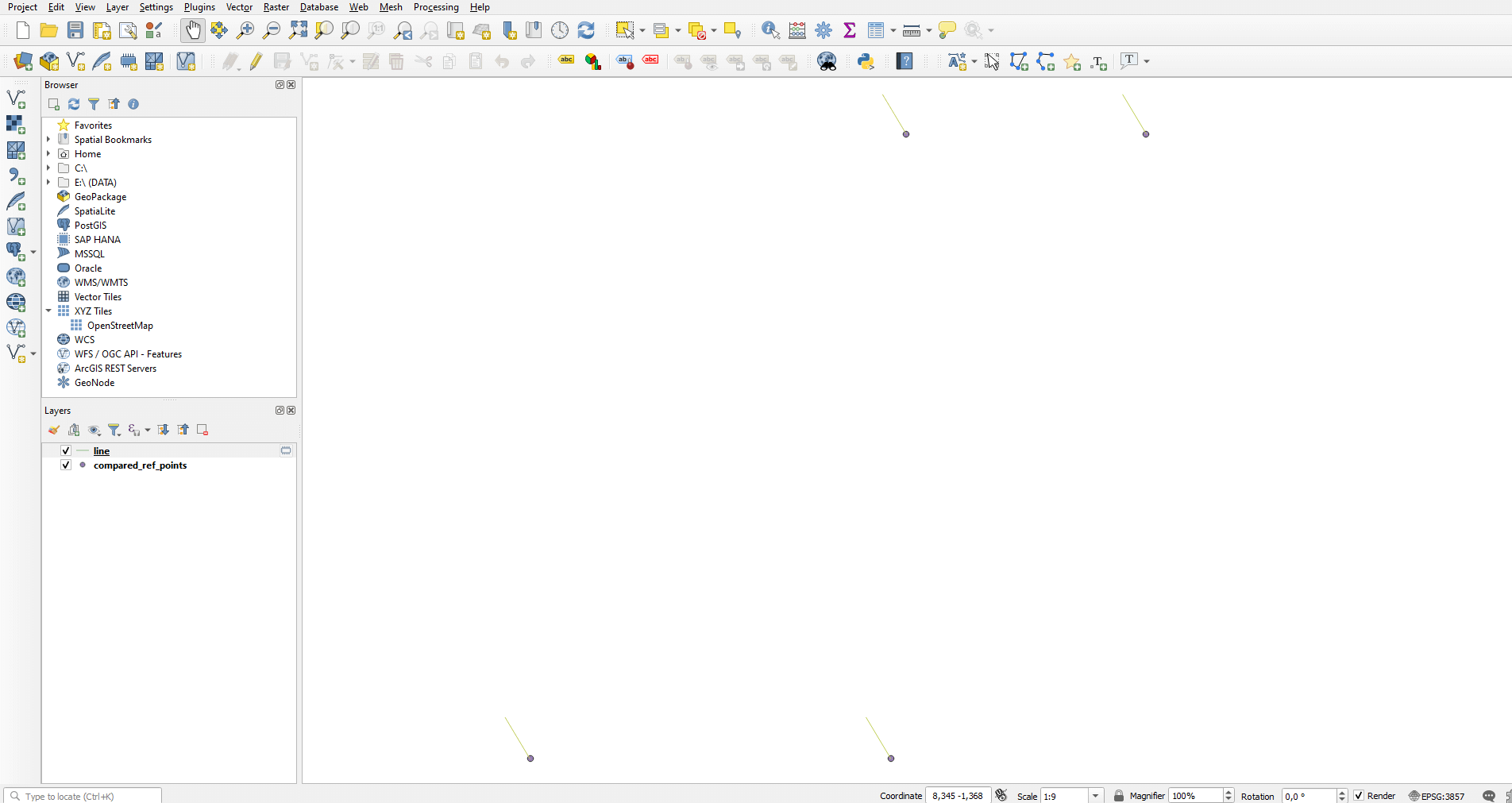
Change the variables if needed: change the column names, or if you aren’t working in Pseudo-Mercator coordinate system, change the EPSG code. Briefly, the script queries the starting X, Y, Z coordinates from every row of the data table. It creates geometries from these, then does the same with the end point. Finally, it creates the new 3D lines (which illustrates the displacements) into a new virtual layer. If everything seems fine, click on the green triangle shaped “Run Script” button. Don’t worry it won’t destroy the whole world or anything like that.
Close the “Python Console”, we won’t use it anymore. On the map canvas the awaited lines will appear.
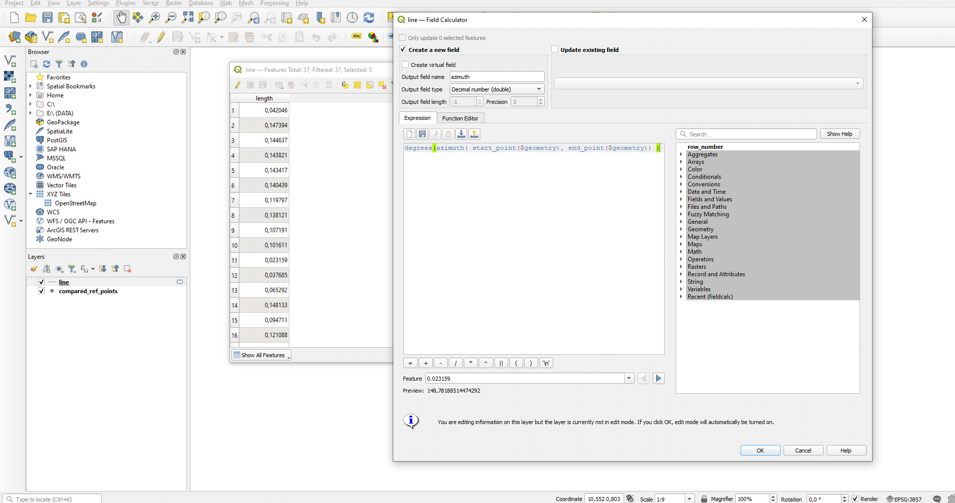
Open the attribute table of the new layer. Add a new column with the “Field Calculator”. Name it “azimuth”. Paste the following command:
degrees(azimuth(start_point($geometry), end_point($geometry)))
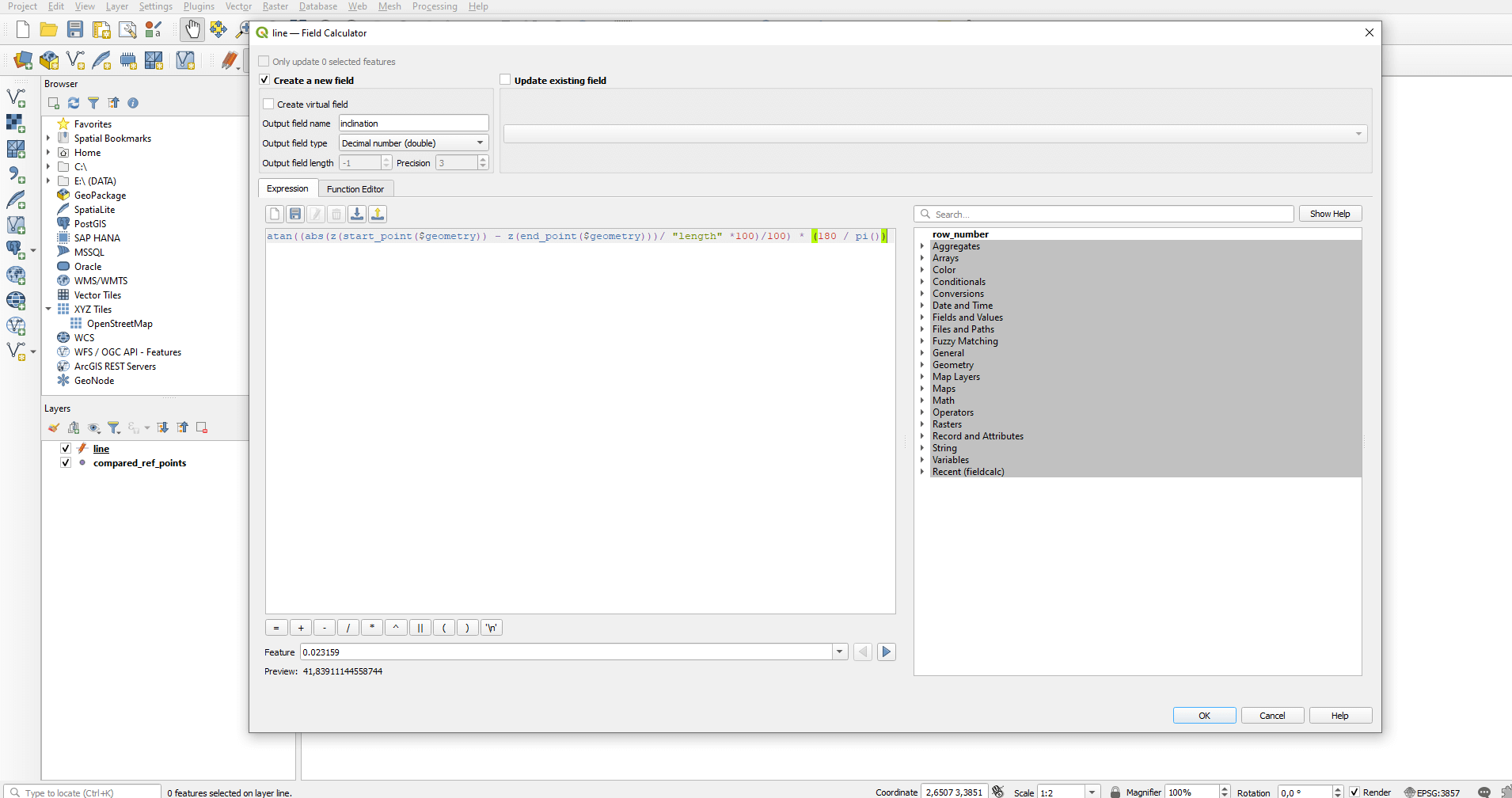
Calculate the angles of inclinations the same way, using “Field Calculator”. Name the new field “inclination”. Paste the following formula:
atan((abs(z(start_point($geometry))-z(end_point($geometry)))/"length"*100)/ 100)*(180/pi())
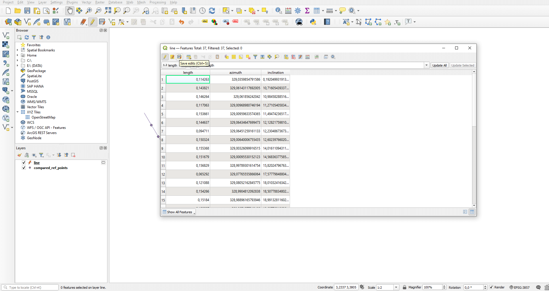
If you have followed the instructions, the data table should look like as shown below. Press the “Save edits” button and close the editing with the pencil shaped icon.
Regarding that this file, which contains the 3D lines, only exists in a virtual memory, I recommend saving it as a real file. Right click to the name of the layer and choose the “Export” option, then the “Save Features As…” command.
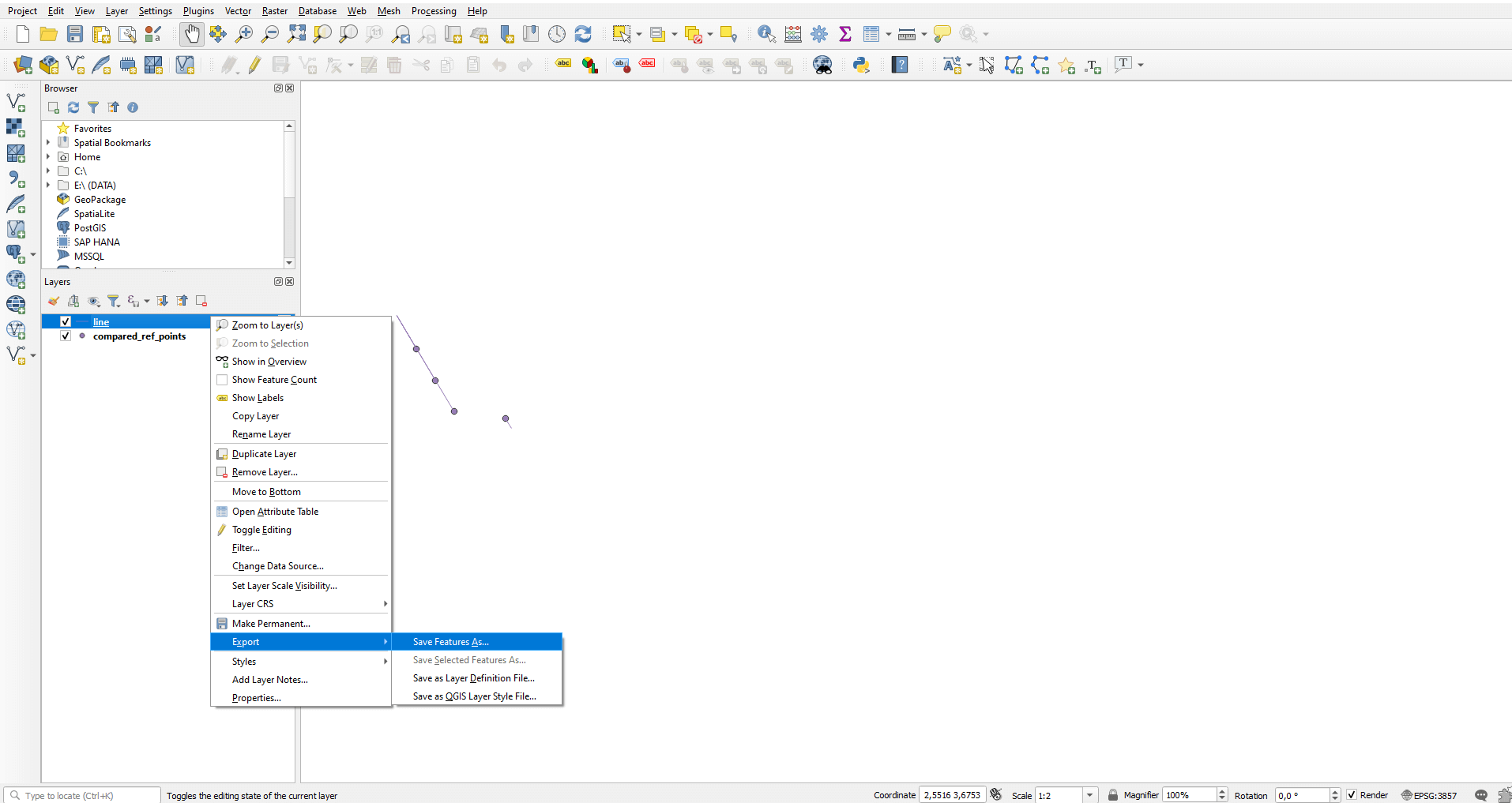
In the pop-up window you can choose the file location, the coordinate system and the format of the 3D lines.
SURFACES
In this chapter I do the same process as shown before with the distance measuring of the surfaces exported from CloudCompare. I want to present how much more data we create when we measure distances between surfaces. With this mass of data, we can get started when making a statistical report.
VISUALIZING DATA
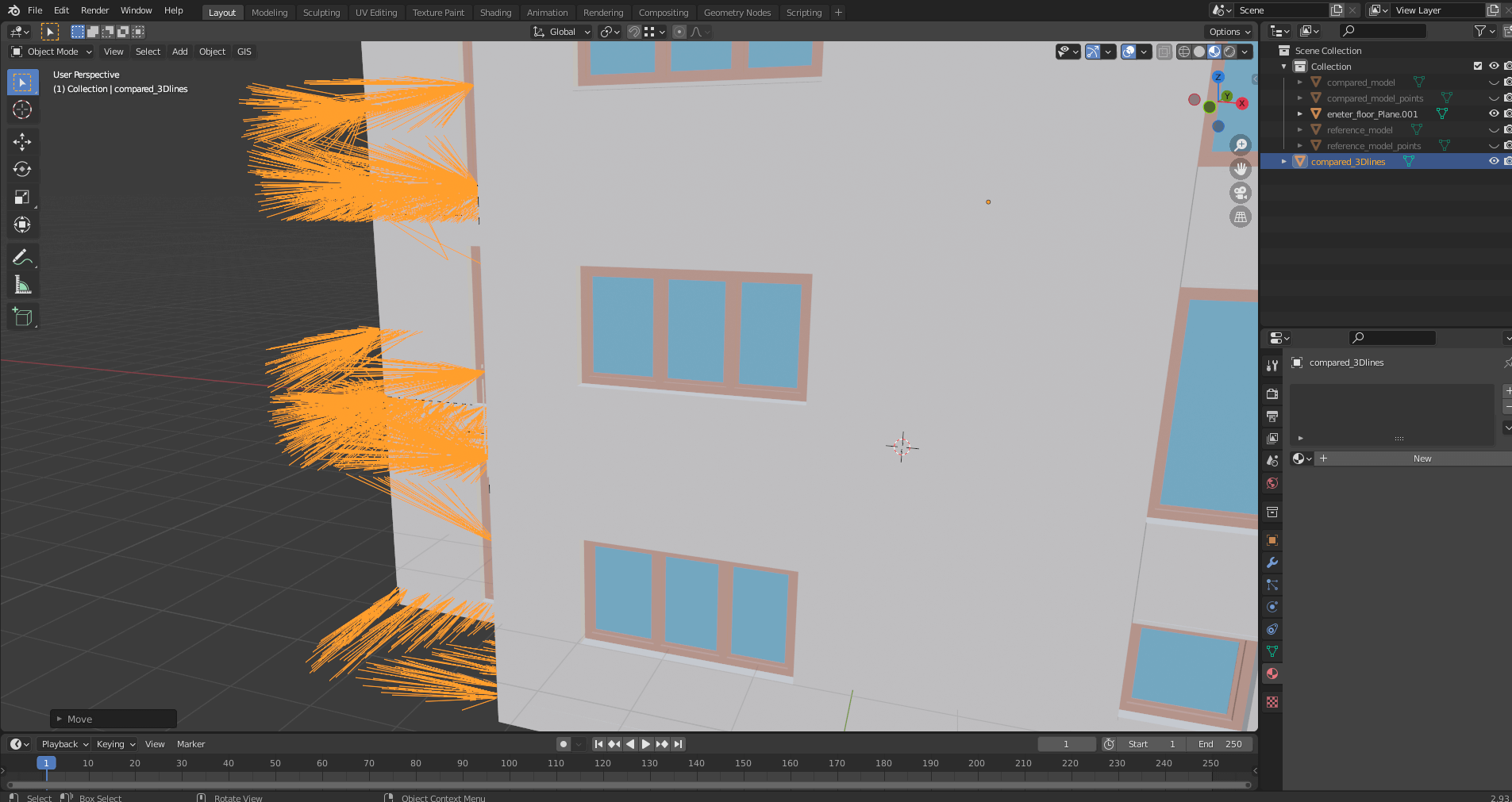
If you have a minute, I will show you a visualizing method with a cool output. Get back to Blender and import the exported 3D lines and the Reference and Starting models using BlenderGIS. It’s clearly visible that we have solved the problem presented at the beginning of the article. We have analyzed the spatial changes of the same identifiable points.
The vector lines of the distance measurements between the surfaces can also be examined nicely. However, even at this stage it’s clear that some points didn’t fall into the right place. Because of that, this data can only be used carefully and with strict controls. Filter these wrong data if needed.
CLOSING THOUGHTS
I think this article will help you to solve a similar distance measuring task. However, I have to emphasize that this is an expert job, so it requires a proper perspective. By that I mean you should always think through if your data matches with the real-life phenomenon. Don’t blindly believe that software functions return perfect results. How to do that? Dive deep into the software and the functions you use to learn how they work. So, you will always be aware of their limits and what they’re made for. Always think through (from the project’s aspect) the methods you need to use, and calculate with the possibility of errors. If you know what errors might occur, it will be easier for you to find a solution.
Did you like what you read? Do you want to read similar ones?
If you really like what you just read, you can share it with your friends via our social media sites. 🙂